Ex. 1: Minimum Fluidization

In this first simple example, we’ll use a pre-defined MFiX case contained in the GUI to examine some of the MFiX-Nodeworks interactive features by tracing out a \(U_{mf}\) curve.

Create MFiX case

1. First enter your local MFiX environment and launch a new instance mfix -n.

2. Navigate to the New pane in the File Menu and select the case FluidBed_2D, give the project name and location and hit OK to create the case.

3. In order to trace out \(U_{mf}\), we’ll need to adjust the inlet velocity. Although we could just find the MFiX intrinsic variable name in the Nodeworks dictionary, let’s give it something more identifiable. Navigate to the Boundary conditions pane, and select the region named Bottom Inlet. Right click on the Y-axial velocity entry, select Create Parameter and give the inlet velocity a meaningful name. In the following, we’ll name it inflow.

4. Now, we need to create a monitor to record the pressure drop in the bed. We want to compute the averaged the bed gas-phase pressure near, but not at, the inlet. First, in the Regions pane, click to add a new region. We’ll call this region dy1, which will range in X from xmin to xmax and in Y from 0.01 to 0.01, i.e., uniform at one vertical grid spacing \(\Delta_y\). The case is 2-D so the Z range of the region can be left at zero.

5. Now we can go to the Monitors pane, click the button to create a monitor. We’ll set the monitor type to average then highlight the dy1 region we just created and hit OK. Set the Type to Average and the Filename base to DPbed. The default Write interval is likely sufficient, but we’ll reduce it to 0.01 (s) for slightly more temporal resolution. At a minimum, make sure to check Pressure as the monitor data to write.

6. Before moving to nodeworks make sure to save the case. If running the GUI without a distributed default solver, we recommend also building a project solver at this time.

Sweep parameter space

1. Now that we have a base case, we can perform a parameter with the surrogate modeling and analysis tools available in Nodeworks. In this example, we just have a simple 1-D parameter space in the parameterized inflow variable. However, the general procedure can be followed for more complex sampling of higher-dimensional parameter spaces. To begin, navigate to the Nodeworks tab in the bottom toolbar to open up a blank Nodeworks worksheet.

2. Right click on the sheet and add a Design of Experiments node from the Surrogate Modeling and Analysis node collection in the node library.

3. Click in the Variable tab to add a new variable.

4. Now, we want to vary the gas inlet velocity which was parameterized as inflow or your user specific name. Click on the variable entry and type the parameterized variable name. You should see the variable appear in the tab-completion drop down menu as you type.

5. (Optional) Label the units as (m/s).

6. Now we need to determine how many points (or samples) to run and over what range. We’ll sweep from zero (exclusively) to 0.20 (m/s), by intervals of 0.01 m/s. Set from to 0.01, to to 0.12 and levels to 10.

7. Now navigate to the Design tab. Set the Method to factorial and check the Use variable specific levels option. Alternatively, the global levels could be entered here on the Design tab. Click the Build button to generate the samples and verify by the table entries or in the Plot tab that the desired points are set.

8. Navigate to the Run tab and set the prefix of the subdirectories to umf. Click Over-Write to create the subdirectories, each containing an individual .mfx file. You should notice messages in the console window indicating that the twelve .mfx files have been exported from the master file (base case).

9. Now we are ready to run the jobs. Click on the Run button and select either your distributed default mfixsolver or local project build and then click Run in the Run solver pop-up window. You should notices additional messages in the console window announcing running jobs.

Warning

In some distributions, Nodeworks can not determine the job ID leaving the MFiX server waiting for pid. If this occurs, please manually check if jobs are running and when they have completed. Additionally in Step below use the Output Selection option All Runs.

Determine \(U_{mf}\)

1. After the jobs have completed, right click on the Nodeworks worksheet and add a Monitor Reader node from the MFIX collection in the node library. Set the Monitor to the DPbed monitor we created previously and the Variable to p_g. We will neglect the first 1 (s) of simulation as transient data and average in time From 1 To 2 (s). Set the data Reducer to mean.

2. Add a Range node from the numpy collection in the node library. Set the start, stop and step to 0.02, 0.21 and 0.02, respectively.

3. Add a Plot node from the matplotlib collection in the node library.

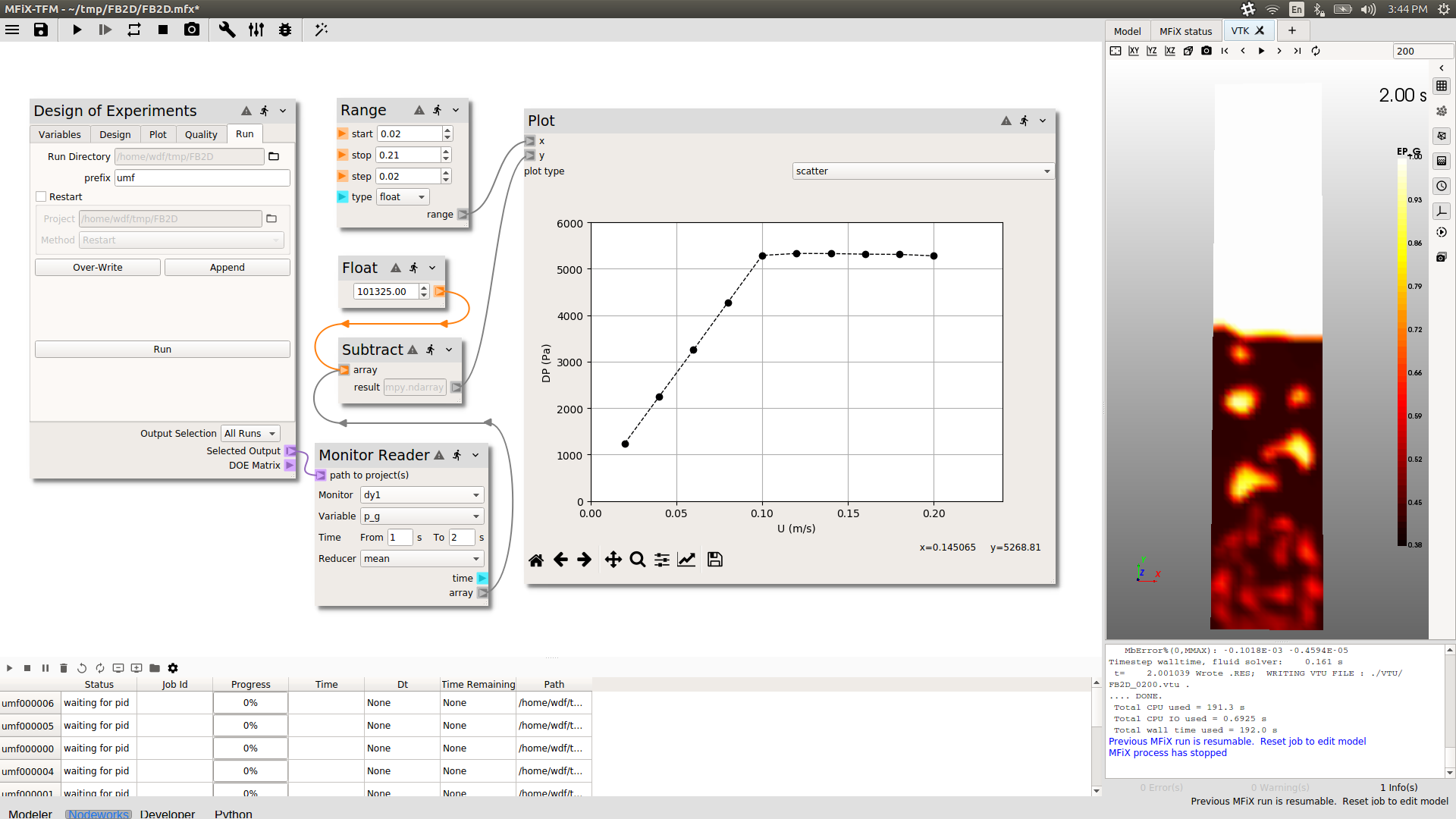
4. Connect the nodes. Set the Output Selection to completed or all runs and connect the Selected Output terminal of the DOE node to the path to project(s) terminal of the Monitor Reader node. Connect the array terminal of the Monitor Reader to the y and the range terminal to the x terminal of the Plot node.

5. Finally, press to run the sheet and generate the \(U_{mf}\) curve as shown below, predicting a value of approximately 10 (cm/s).

Note

As is, the bed pressure is not a pressure drop as the outlet (atmospheric) pressure is included. There are several ways to remove the outlet pressure, one of which would be to create a second monitor near the outlet. However, since the outlet pressure is a constant across all runs, this can be handled in Nodeworks by adding a Subtract node–make sure to use the numpy version–and a Float node with a value of the outlet boundary condition of 101325 Pa. Connect the monitor then the float to the subtract node and then the subtract node to the plot node in order to arrive at the Umf plot shown above.