Neural Network Regressor
The Neural Network Regressor node has been designed to mimic the
Response Surface node, but tailored to construct neural networks. This node
supports multiple continuous input variables and only one response variable.
Currently, the node uses PyTorch and will
automatically use the GPU if the drivers are installed correctly. The resulting
neural network can be used with the other from the
surrogate modeling and analysis toolset such as the General Optimizer
node, Forward Propagation node, Sensitivity Analysis node, and the Residual Function node.
The main controls of the node persist at the bottom, consisting of Train,
Import, and Export buttons. The Train button will start training
the neural network. The Import button will open a browse dialog that can be
used to select an exported neural network model to load. Finally, the Export
button will open a browse dialog that can be used to export the trained model.
Note
If the Neural Network Regressor node does not appear in your list of
available nodes, please install PyTorch using PyTorch’s install instructions
located here.
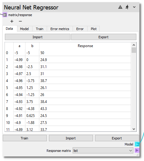
Data
In the Data tab the required parameter input and corresponding full model
response values are entered into the node for the construction of the response
surface. There are two ways in which the required data can be input. In a
typical workflow, the input matrix (typically from a Design of Experiments node) and
the corresponding model response (typically from a code node) are connected
to the matrix/response terminal. Alternatively, if the data has been
generated externally or exported from Nodeworks nodes and agglomerated into a
single table, the Import button at the top of the table can be used to
read in a csv file.
Once the input and response data has been loaded into the Data tab, it can
be sorted by individual input variables or the (full model) Response. The table
can be returned to the original index order by right clicking and
selecting clear sort. The right click menu also offers the capability to
Exclude or Include specific entries.
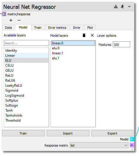
Model
The structure of the neural network is defined on the Model tab. Layers can
be clicked and dragged from the Available layers list to the
Model layers list. Layers can also be added by double clicking layers in the
Available layers list. The Available layers list can also be filtered by
entering text in the Search field. Individual layer options can be edited
by selecting a layer in the Model layers list and changing the values in the
widgets that appear under the Layer options.
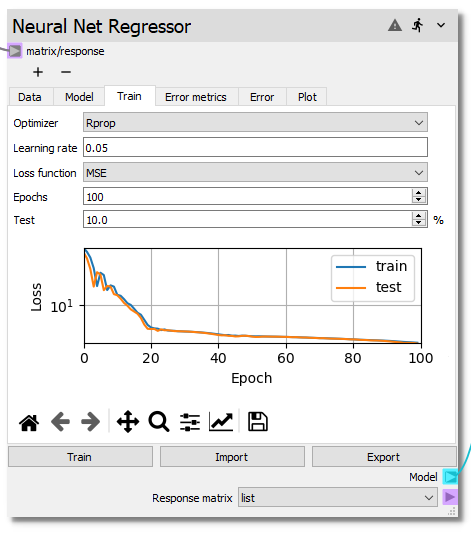
Train
Training parameters are selected on the Train tab. This includes the number
of epochs and the percentage of samples to hold out for cross validation. During
training, the plot will update, display the current epoch error metric for both
the training data and the test data (if the cross validation percent is greater
than 0).
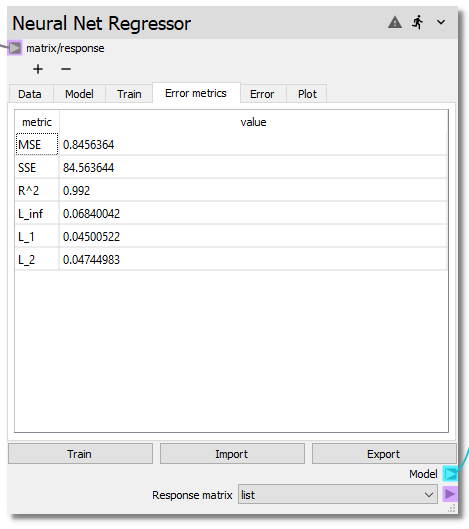
Error Metrics
The table on the Error Metrics tab shows several quantitative error metrics
that can be used to assess the fitness of the trained neural network.
RSM Error Metrics:
MSE- Mean Squared Error
SSE- Sum of Squared Error
R^2- R squared
L_inf- L_infinity norm
L_1- L_1 norm
L_2- L_2 norm
The error metrics operate on either the full dataset or the out-of-sample subset for
cross validation.
In cross validation, a subset of the dataset is withheld from the training of the
model. By default, 10 percent of the dataset is withheld as
Cross validation points. When cross validation is active, the RSM Error Metrics:
only apply to the withheld points. Without cross validation, the RSM Error Metrics:
apply to the whole dataset.
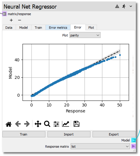
Error
The difference between the model and the data is visualized in the
Error tab. The discrepancy for a given model can be viewed
in three different forms selectable from the Plot dropdown menu:
parityplot
errorploterror
histogram
As in the Plot tab of this and the Response Surface node, points can be
highlighted by holding select and dragging the cursor. Highlighted points can be
excluded (and included if previously excluded) from the fit of the model.
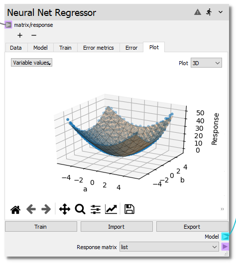
Plot
The trained model can be visualized in either 3D or as a contour plot,
as shown below, in the Plot tab. If more than two input variables are used, the
variables used for the X Axis and Y Axis become selectable from dropdown
menus below the plot. For the variables not plotted on either the X Axis or
Y Axis, the surface will be evaluated at the center of the variable range.
The user can change these values by selecting the variable values dropdown
and adjusting either the slider or entering a new value in the line edit.
Response data points are selectable and can be excluded from the fit or shown in
the Data table from the right click menu.