Response Surface
After the full model has been run and the responses collected at the sampled points, the
responses can be interpolated into a Response Surface. The response surface maps
continuous input parameters into a continuous (or at least piece-wise continuous)
output (response), thus acting as a surrogate model for the full model evaluation.
The basic functionality of the Response Surface node is outlined below and used
extensively in the Examples.
Data
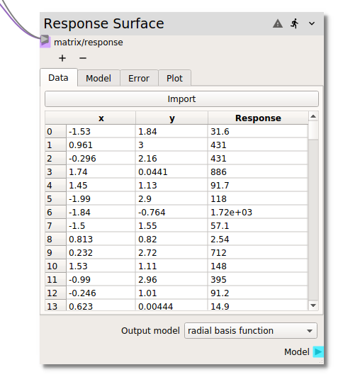
In the Data tab the required parameter input and corresponding full model response values
are entered into the node for the construction of the response surface. There are two ways in
which the required data can be input. In a typical workflow, the input matrix (typically from
a Design of Experiments node) and the corresponding model response (typically from
a code node) are connected to the matrix/response terminal as shown in the figure above.
Alternatively, if the data has been generated externally or exported from Nodeworks nodes and
agglomerated into a single table, the Import button at the top of the table can be used to
read in a csv file.
Once the input and response data has been loaded into the Data tab,
it can be sorted by individual input variables or the (full model) Response. The table can
be returned to the original index valued order by right clicking and selecting clear sort.
The right click menu also offers the capability to Exclude or Include specific
entries.
Preprocessing
With some response surface models, it is important to preprocess the input samples so one variable does not dominate the objective function and make the estimator unable to learn from other features correctly as expected. The following preprocessors are available and are applied to the training data used by all the models:
none- Don’t use any preprocessing [default]zero mean and unit variance- Standardize features by removing the mean and scaling to unit variance. Uses StandardScaler from scikits-learn.Scale- Scales all the variables individually so they fit in the provided range.normalize- Normalize samples individually to unit norm. Uses Normalizer from scikits-learn.quantile transform- Transforms the features to follow a uniform or a normal distribution. Uses QuantileTransformer from scikits-learn.power transform- Transforms features to make data more Gaussian-like. Uses PowerTransformer from scikits-learn.
Model
There are several response surface modeling choices available in the Model tab drawing from
the scikits-learn and scipy libraries. Current modeling options include:
With so many different modeling options, determining which particular model is best, or even
which sub-options of a given model are best, can be a challenging task. Several features within
the Response Surface node have been included to help with model selection.
The following section covers the Error tab which provides graphical representation
of the surrogate model error, i.e., the difference between actual (full) model response
and the response surface at the corresponding input values. The table on the Model tab
shows several quantitative RSM Error Metrics:
MSE- Mean Squared Error
SSE- Sum of Squared Error
R^2- R squared
L_inf- L_infinity norm
L_1- L_1 norm
L_2- L_2 norm
The error metrics operate on either the full dataset or the out-of-sample subset for
cross validation.
In cross validation, a subset of the dataset is withheld from the fitting of the
response surface. By default, 10 percent of the dataset is withheld as
Cross validation points. When cross validation is active, the RSM Error Metrics:
only apply to the withheld points. Without cross validation, the RSM Error Metrics:
apply to the whole dataset.
Since each cross validation attempt pulls random samples for testing, it can be difficult to discern improvements in the fit quality when manually adjusting model parameters. To help with this, the fitting process can be repeated multiple times by entering a value in the repeats field greater than 1.
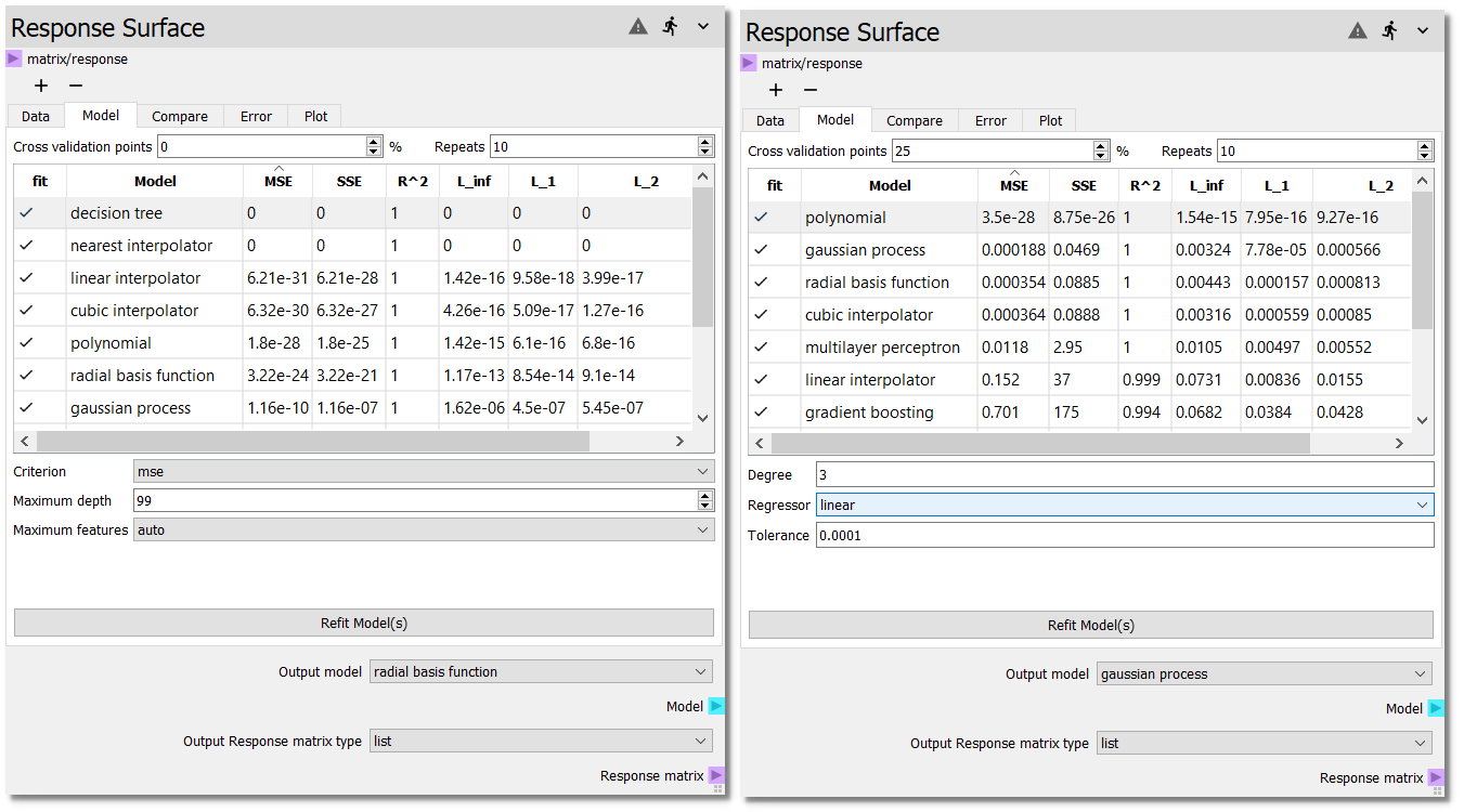
The figure above shows several Model surrogate candidates without cross
validation on the left and with 25% cross validation on the right. Without cross
validation six models show near zero error (to double precision). However, these
interpolators are designed to agree with the model at the sampled points. But
how do these surrogates perform over the entire design space, i.e., in between
the sampled points? One way to test this is with cross validation. When the
models are fit to only 75% of the samples, we see that the polynomial, gaussian
process (GP), and radial basis function (RBF) models have better predictive
accuracy of the 25% hold out data. The cross validation points can also be
used to fine tune model parameters. After activating new models or changing
model options, the error metrics can be reassessed by hitting the
Refit Model(s) button. The Refit Model(s) button can also be used
without changing any modeling options to simply re-draw the
Cross validation points, which are drawn at random from the full data set.
Warning
After assessing the performance of different surrogate models with the
RSM Error Metrics and the Error plots, make sure to
return to the Model tab, set the Cross validation points to 0
and hit the Refit Model(s) button to re-fit the surrogate to the
full dataset before use in downstream analysis nodes.
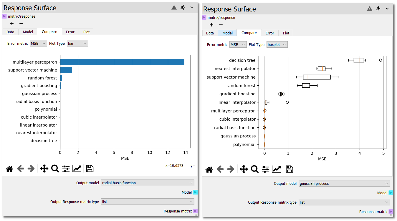
Compare
To visually compare the performance of the surrogate models, the compare plot plots the error metrics displayed in the model table. There are three plotting options for the error metrics. If the number of repeats is greater than 1, then the standard deviation of the error metrics will be added to the bar plot and the boxplot and violin plots will be selectable.
Error
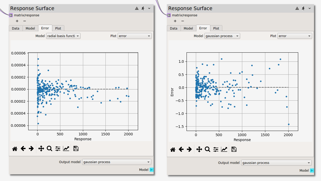
The difference between the surrogate model(s) and the data is visualized in the
Error tab. If more than one surrogate model has been fit, they can be selected
from the Model dropdown menu. The discrepancy for a given model can be viewed
in three different forms selectable from the Plot dropdown menu:
parityplot
errorploterror
histogram
As in the Plot tab of this and the Design of Experiments nodes, points can be highlighted
by holding select and dragging the cursor. Highlighted points can be excluded
(and included if previously excluded) from the fit of the response surface models.
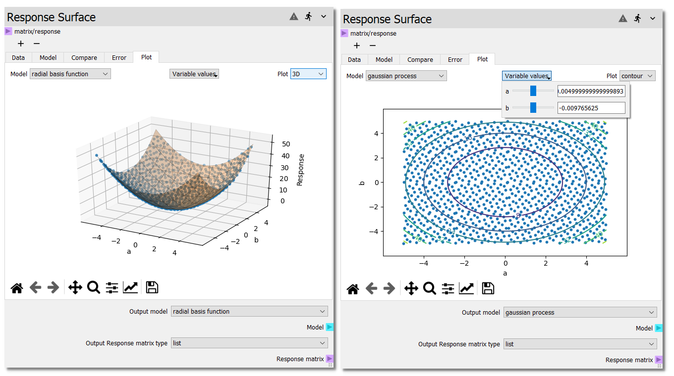
Plot
The different models can be visualized in either 3D or as a contour plot,
as shown below, in the Plot tab. If more than two input variables are used, the
variables used for the X Axis and Y Axis become selectable from dropdown
menus below the plot. For the variables not plotted on either the X Axis or
Y Axis, the surface will be evaluated at the center of the variable range.
The user can change these values by selecting the variable values dropdown
and adjusting either the slider or entering a new value in the line edit.
Response data points are selectable and can be excluded from the fit or shown in
the Data table from the right click menu.
Output
Located at the bottom of the node below all of the tabs is the Output model selection.
If the models become computationally intensive, it is recommended that all but the desired
model be deselected from the Model tab. However, if it is desired to use more than one
surrogate model for analysis in downstream nodes, the different models can be toggled with
the Output model dropdown.
Warning
Remember to return to the Model tab, set the Cross validation points
to 0 and hit the Refit Model(s) button to re-fit the surrogate to the
full dataset before continuing.