4.6. Solids
The solids pane is used to set solids phases material properties. The “Materials” tab sets material properties shared by most models (TFM, DEM and PIC). Specific settings for each model are accessed through their respective tabs (TFM, DEM, or PIC).
4.6.1. Creating a Solids phase
A new solids phase is created by clicking the add button,  ,
at the top of the solids table. This will create a new entry
in the table. The table summarizes all defined solids phases
by listing the name, model, particle diameter and density.
A blank entry in the density means the particle density is
variable (it depends on its chemical composition).
,
at the top of the solids table. This will create a new entry
in the table. The table summarizes all defined solids phases
by listing the name, model, particle diameter and density.
A blank entry in the density means the particle density is
variable (it depends on its chemical composition).
- Name
The name used to refer to the solids phase in the GUI. By default, the solids phase is called “Solid” followed by its assigned phase number. The phase number is incremented every time the
button is pressed.
The solids phase name may be renamed for convenience (optional).
This name will appear in other panes or tabs when referring to the
solids phase (say while setting initial or boundary conditions).
Model (read only)
The modeling approach used to represent the solids phase. Available options include TFM (Two-Fluid Model), DEM (Discrete Element Model) and PIC (Particle in Cell). The setting is currently locked (the same solid model must be used for all solids phases), and mirrors the solver selection in the Model Setup pane.
4.6.2. Deleting a Solids phase
A solids phase can be deleted by selecting it (click on its name in the
solids table) and clicking the remove button,  ,
at the top of the solids table. If the solids phase is used in the
model with a non-zero solids fraction (say in an initial or
boundary condition), the deletion will need to be confirmed by the user.
If confirmed, the deleted solids volume fraction will be assigned
back to the fluid phase.
,
at the top of the solids table. If the solids phase is used in the
model with a non-zero solids fraction (say in an initial or
boundary condition), the deletion will need to be confirmed by the user.
If confirmed, the deleted solids volume fraction will be assigned
back to the fluid phase.
4.6.3. General Solid Model Options
- Solve momentum equation (TFM only)
By default, all momentum equations are solved. Individual momentum equations may be disabled by toggling the check box.
- Solve species equations
By default, species transport equations are not solved for the solids phase. If species equations are enabled, species will need to be added to the solids phase using the solids species tool. ADD REF
4.6.4. Solids phase Material Properties
Some material properties are only needed for a specific solid model or when the energy or species equation is solved.
- Diameter \((m)\)
The initial particle diameter. It will remain constant for non-reactive flows, and for reactive flows with a variable density. If the density is constant, and chemical reactions take place, the particle diameter will vary to reflect particle mass gain/loss.
- Density \((kg \mathbin{/} m^3)\)
The particle density can be set as:
Constant:
A positive (non-zero) number must be provided.
The diameter may change due to chemical reactions.
Variable:
The density is computed from particle’s mass and volume.
The particle mass is function of the particle’s chemical composition.
A variable density can only be used if species equations are solved.
- Viscosity \((Pa \cdot s)\) TFM only
It may be specified using one of the following approaches:
Constant:
A positive (non-zero) number must be provided.
Continuum Solids stress Theory
User-Defined Function (UDF)
A custom equation of state must be provided in the usrproperties.f
A custom solver must be built.
- Molecular weight \((\frac{kg}{kmol})\)
It may only be specified using the following approach, and is only used when Energy and solids species equations are solved:
Mixture
Requires species be used to defined the solid.
Requires species mass fractions be specified for the whole domain and all flow boundary conditions
- Specific heat \((\frac{J}{kg \cdot K})\)
It may be specified using one of the following approaches (only used when Energy and species equations are solved):
Constant:
A positive (non-zero) number must be provided.
Mixture
Requires species be used to defined the fluid.
Requires species mass fractions be specified for the whole domain and all flow boundary conditions
User-Defined Function (UDF)
A custom equation of state must be provided in the usrproperties.f
A custom solver must be built.
- Thermal conductivity \((\frac{W}{m \cdot K})\)
It may be specified using one of the following approaches:
Constant:
A non-negative number must be provided.
Temperature-Dependent
Option available for TFM only.
Requires solids phase temperature be specified for the whole domain and all flow boundary conditions.
User-Defined Function (UDF)
Option available for TFM only.
A custom equation of state must be provided in the usrproperties.f
A custom solver must be built.
- Emissivity \((-)\) DEM only
The emissivity of the DEM solids phase. Leaving it blank or setting a zero value turns radiation off.
- Parcel weight \((-)\) PIC only
A default parcel weight (number of particles per parcel) may be specified for convenience (default value of one). it is used to define a default statistical weight for parcels in initial conditions regions and mass inflows. Instead of defining the same parcel weight in every initial condition and mass inflow, this default value is automatically applied. The default value can be overwritten where needed.
4.6.5. Solids Model Species
Specie that comprise the solid phase are summarized in the species overview
table. New species are added by clicking the add button, , at the top
of the species table.
4.6.6. Advanced settings
- Disable close pack (TFM only)
Options to enable/disable a TFM phase from forming a packed bed. This is typically used to make the solids phase behave as a liquid phase.
- Enable added mass force (TFM only)
Options to enable/disable the added (or virtual) mass force in a TFM phase. This tends to stabilize bubbly gas/liquid flows.
4.6.7. TFM Settings
Specific Two-Fluid Model settings are accessed from the TFM tab.
- Packed bed void fraction \((-)\)
The void fraction at close pack.
- Viscous stress model
The solids phase stress model. Options include the algebraic formulation or various kinetic theories requiring solving a Partial Differential Equation for the granular energy:
Algebraic Formulation [DEFAULT]
Lun et al, 1984
Iddir & Arastoopour, 2005
Simonin, 1996 (requires k-ε turbulence enabled)
Cao & Ahmadi, 1995 (requires k-ε turbulence enabled)
Garzo and Dufty, 1999 (monodisperse system only)
Garzo, Tenneti, Subramaniam, Hrenya, 2012 (monodisperse system only)
Garzo, Hrenya and Dufty, 2007 - Requires at most two solids phases - Requires Wen-Yu or HYS drag model - Selection not available with added mass force
- Frictional stress model
Schaeffer model [DEFAULT]
Srivastava and Sundaresan
Only solids pressure
- Solids volume fraction at onset of friction \((-)\)
The minimum solids fraction above which the Srivastava and Sundaresan model sets in.
- Particle-particle restitution coefficient \((-)\) :
The coefficient of restitution for particle-particle collision.
- Interphase friction coefficient \((-)\) :
The coefficient of friction between particles of two solids phases.
- Angle of internal friction \((\deg)\) :
The angle of internal friction. The plastic regime stress can be turned off by setting this value to zero.
- Radial distribution function
Carnahan-Startling (only option for monodisperse systems)
Lebowitz (default for polydisperse system)
Mansoori (polydisperse system)
Modified Lebowitz (polydisperse system)
Modified Mansoori (polydisperse system)
- Stress blending
The blending function used to smooth transition around the packed bed volume fraction. It requires the Schaeffer frictional stress model.
None [DEFAULT]
Hyperbolic Tangent
Sigmodial
- Segregation slope coefficient \((-)\)
Coefficient used in calculating the initial slope in segregation for polydisperse systems.
- Max packing correlation
The correlation used to compute the maximum packing for polydisperse systems:
Constant [DEFAULT]
Yu & Standish
Fedors & Landel (only with two solids phases)
- Excluded volume in Boyle-Massoudi stress \((?)\)
The excluded volume in Boyle-Massoudi stress. It is only used with the algebraic formulation of viscous stress model (optional).
4.6.8. DEM Settings
Specific Discrete Element Model settings are accessed from the DEM tab.
- Enable automatic particle generation
Initialize particle location and velocity based on information from Initial Condition regions. If this option is disabled and any initial condition uses a non-zero solids volume fraction, the user will be prompted to turn on this option. Disabling this option will read initial particle location and velocity from a user generated text file (particle_input.dat) that must be saved in the project directory.
- Data file particle count \((-)\)
The number of particles read from particle_input.dat file when the automatic particle generation is turned off. This number must be smaller or equal to the number of lines in the file.
- Particle Size Distribution (PSD)
A series of PSDs can be defined to be used in an initial condition region or a mass inlet boundary condition. A PSD represents the number of particles having a given size. It is currently a number-based (not volume-based) distribution. A new PSD is created by clicking the add button,
, and entering the PSD parameters. The PSD can follow
a Normal or Log-normal distribution. There is an option to load a text file containing a custom PSD.
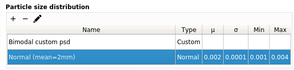
Fig. 4.1 Particle Size Distribution table.
Initially, the table will be empty. Double click on one row to edit a PSD, Click on to remove a PSD
from the table.
First, enter a descriptive name for the PSD and choose the PSD type.
Parameters for the Normal and Log-normal distribution are:
Mean particle diameter
Standard deviation
Minimum diameter , used to clip the distribution and avoid extremely small particles
Maximum diameter , used to clip the distribution and avoid extremely large particles
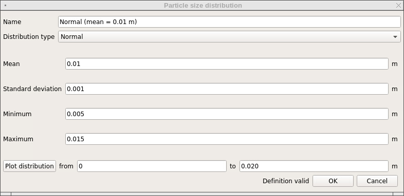
Fig. 4.2 Example of a Normal Particle Size Distribution definition.
Custom PSDs will read the distribution from a text file. It can be edited through any text editor including the GUI built-in editor. The PSD custom file is organized as follows:
The figure below shows an example of a custom PSD file. Only the first few lines are shown.
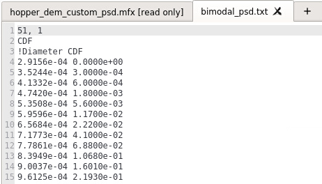
Fig. 4.3 Example of a Custom file used to define a Particle Size Distribution.
Once the parameters are defined, the PSD can be plotted by clicling the ‘Plot distribution’ button.

Fig. 4.4 Plotting a Particle Size Distribution.
- Integration method
The DEM time stepping scheme when integrating the particle trajectories (acceleration to velocity and velocity to position):
Euler [DEFAULT]
Adams-Bashforth
- Collision model
The soft-sphere collision model:
Linear Spring Dashpot (LSD)
Hertzian
- Coupling method
The level of coupling between the gas phase and the solids phase:
One-way coupled
Fully coupled
- Interpolation
The direction of interpolation between field and particle data:
No interpolation
field-to-particle and particle-to-field
field-to-particle only
particle-to-field only
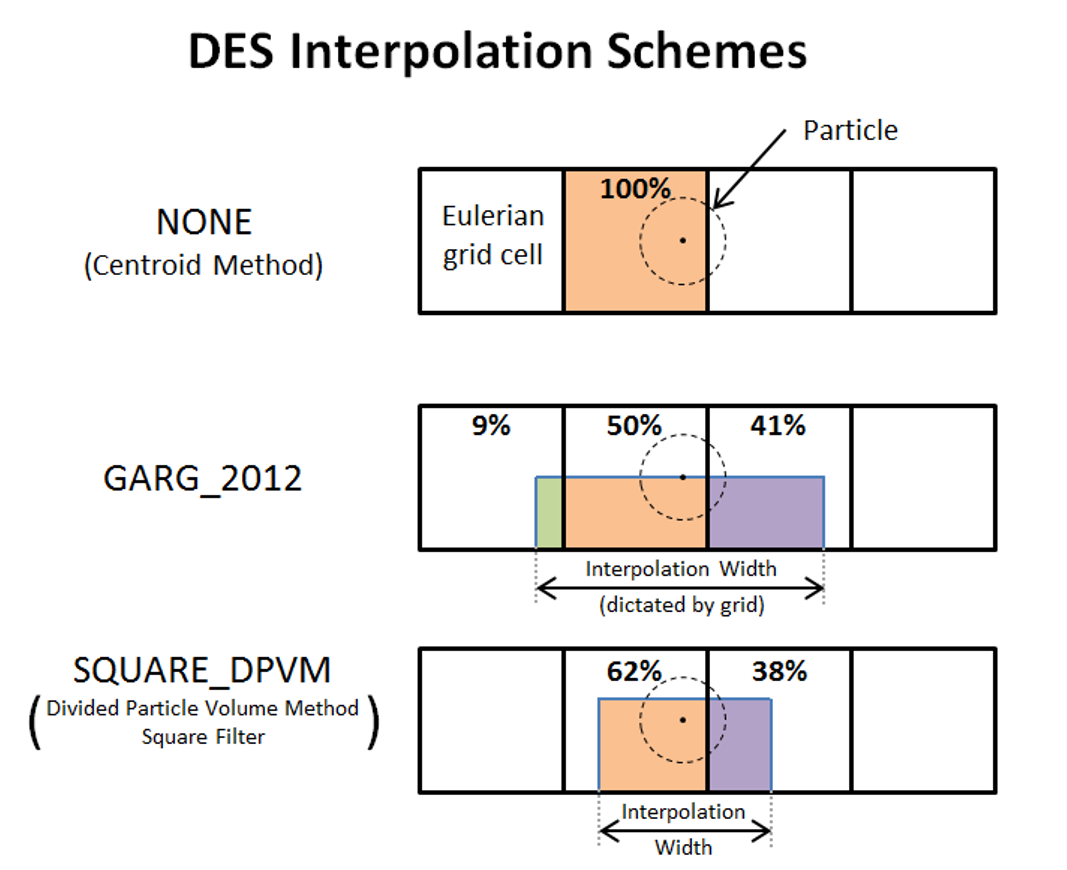
- Scheme
The interpolation scheme:
None (centroid method)
Garg, 2012 (interpolation width is dictated by grid spacing)
Square DPVM (Divided Particle Volume Method), requires an interpolation width.
- Width \((m)\)
The square DPVM interpolation width.
- Enable mean field diffusion
Smooths the disperse phase average fields by solving a diffusion equation.
- Width \((m)\)
The diffusion length scale.
- Enable explicit coupling of interphase quantities
Option to explicitly couple the fluid and solids hydrodynamics.
- Friction coefficient \((-)\)
The particle-particle and particle-wall Coulomb friction coefficient. This is required for both the LSD and Hertzian collision models.
- Normal spring constant \((\frac{N}{m})\)
The particle-particle and particle-wall normal spring constant (LSD collision model).
- Spring norm/tan ratio \((-)\)
The ratio of normal to tangential spring constants for particle-particle and particle-wall (LSD collision model).
- Damping norm/tan ratio \(()\)
The ratio of normal to tangential damping factors for particle-particle and particle-wall (LSD collision model).
- Young’s modulus \((Pa)\)
The wall and particles (one entry per phase) Young’s modulus (Hertzian collision model).
- Poisson’s ratio \((-)\)
The wall and particles (one entry per phase) Poisson’s ratio (Hertzian collision model).
- Restitution coefficients (normal) \((-)\)
The list of normal restitution coefficients for particle-wall and particle-particle interaction. The particle-particle entries are arranged into a symmetrical matrix. The diagonal terms and the upper side of the matrix need to be filled. There is one entry per phase for the particle-wall coefficient. This settings is required for both the LSD and Hertzian collision models.
- Restitution coefficients (tangential) \((-)\)
The list of tangential restitution coefficients for particle-wall and particle-particle interaction. The particle-particle entries are arranged into a symmetrical matrix. The diagonal terms and the upper side of the matrix need to be filled. There is one entry per phase for the particle-wall coefficient. This settings is only required for the Hertzian collision model.
- Cohesion model
Toggles the van der Waals cohesion model. When turned on, additional parameters need to be set (see below):
- Hamaker constant \((J)\)
The particle-particle and particle-wall Hamaker constant used in the van der Waals cohesion model.
- Outer cutoff \((m)\)
The particle-particle and particle-wall maximum separation distances above which the van der Waals cohesion forces are set to zero.
- Inner cutoff \((-)\)
The particle-particle and particle-wall minimum separation distances below which the van der Waals cohesion forces are computed using a surface adhesion model.
- Asperities \((-)\)
The mean radius of surface asperities used in the cohesive force model.
- Minimum fluid volume fraction \((-)\)
Threshold used to clip the fluid phase volume fraction (to avoid non-physical values, typically when a particle size is near a small cut cell).
- Neighbor search method
The neighbor search algorithm:
Grid-based
N-Square
- Max steps between neighbor search \((-)\)
The maximum number of DEM iterations between two neighbor searches. The neighbor search may be called earlier if the particle moves a distance greater than a defined quantity (see below).
- Factor defining particle neighborhood \((-)\)
A multiplying factor applied to the particle’s radius to define the region where particle neighbors are searched from.
- Distance/diameter triggering search \((-)\)
The distance a particle can travel before triggering an automatic neighbor search.
- Search grid partition \((-)\)
The number of DEM grid cells in each direction used for the neighbor search. This is an optional setting. If left undefined, the number of cells is computed so that the DEM grid size is three times the maximum particle diameter.
- Enable user scalar tracking
Turns on the tracking of user-defined scalars attached to each particle. When the tracking is enables, the number of scalars (positive integer) needs to be set.
- Minimum conduction distance \((m)\)
The minimum separation distance between particles (used in the particle-fluid-particle conduction model to remove singularity).
- Fluid lens proportionality constant \((-)\)
Constant used to calculate the fluid lens radius that surrounds the particle (used in the particle-fluid-particle conduction model).
- Young’s modulus used to correct DEM conduction \((Pa)\)
The wall and particles (one entry per phase) Young’s modulus used to correct the DEM conduction. These optional input are used with both LSD and Hertzian collision models. Particles are typically made softer to increase the DEM time step. This may lead to inaccurate conduction. If defined, this Young’s modulus will be used to correct the DEM conduction model.
- Poisson’s ratio used to correct DEM conduction \((-)\)
The wall and particles (one entry per phase) Poisson’s ratio used to correct the DEM conduction. These optional input are used with both LSD and Hertzian collision models.
4.6.9. PIC Settings
Specific Particle in Cell settings are accessed from the PIC tab.
Many of the PIC settings refer to the PIC solids stress model, which influences parcel motion:
\(\tau_p=\frac{P_p \epsilon_p^\gamma}{\max[\epsilon_{cp} - \epsilon_p , \delta(1-\epsilon_p)]}\)
- Void fraction at close pack \((-)\)
The void fraction \((\epsilon_{cp})\) at maximum packing.
- Volume fraction exponential scale factor \((-)\)
The empirical exponent \((\gamma)\) on solids fraction in the solids stress model. Typical values are between 2.0 to 5.0.
- Pressure linear scale factor \((Pa)\)
The empirical pressure \((P_p)\) constant in the solids stress model. Typical values are 10 to 1000 Pa.
- Empirical dampening factor \((-)\)
A factor in a restitution coefficient for comparing solids stress with slip velocity. Typical value is 0.85.
- Non-singularity constant \((-)\)
The constant \((\delta)\) to prevent division by zero in solids stress model. Typical value is 1.0E-8.
- Wall normal restitution coefficient \((-)\)
The parcel-wall restitution coefficient for normal velocity component after wall collision.
- Wall tangential restitution coefficient \((-)\)
The parcel-wall restitution coefficient for tangential velocity component after wall collision.
- Solids slip velocity scale factor \((-)\)
A damping coefficient on slip velocity. Typical value is 1.0.