4.11. Monitors
A Monitor is a tool for capturing data from the solver about the model.
Data (such as volume fraction, pressure, velocity, etc.) for a given Region Selection is written to a CSV file while the solver is running.
The number of monitors that can be defined for a project is limited to a maximum of 100.
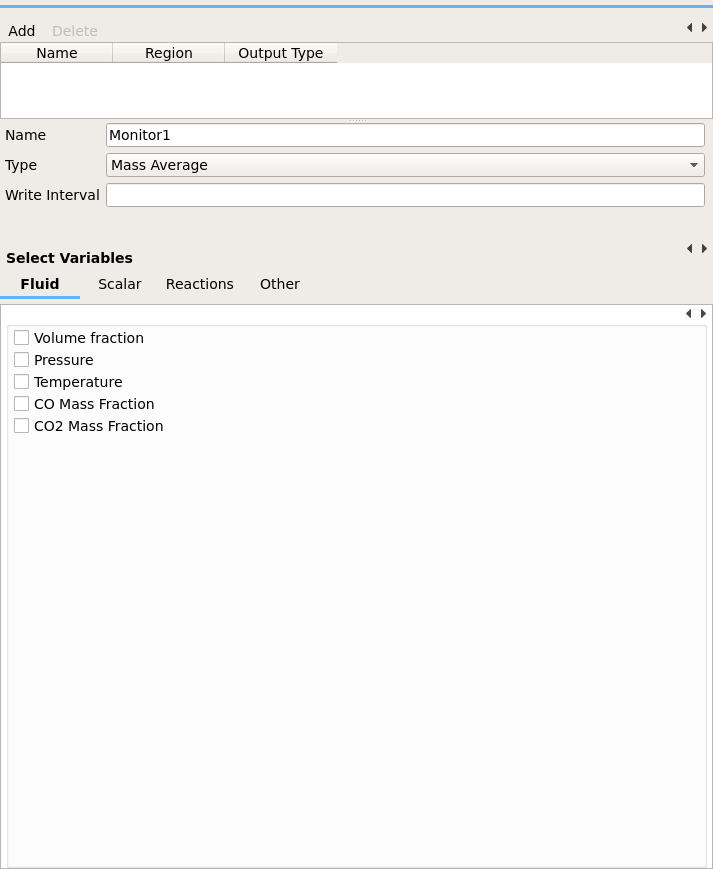
Fig. 4.10 Monitor pane
4.11.1. Region Selection
To define a monitor, there must be a region already defined in the Regions
Pane. Click the  button at the top, which will open a popup
window for selecting the region. A Monitor region is a single point, plane, or
volume. Multiple regions cannot be combined for a monitor, and STL regions
cannot be used for monitors.
button at the top, which will open a popup
window for selecting the region. A Monitor region is a single point, plane, or
volume. Multiple regions cannot be combined for a monitor, and STL regions
cannot be used for monitors.
4.11.2. Monitor Output
- Filename
The monitor output file will have a default name based on the name of the monitor’s region. You can edit the filename of a monitor by selecting the monitor from the list of monitors and changing “Filename base”. The monitor data will be output to the Filename base with the extension
.csv.The monitor output file is in Comma Separated Value (CSV) format. The first line of the file provides header information. For example, running the Silane Pyrolysis tutorial (SP2D) will generate a file
PROBE_SPECIES.csv:# # Run type: NEW # "Time","x_g(1)","x_g(2)","x_g(3)","x_g(4)","x_g(5)","x_s(1,1)","x_s(1,2)" 0.0000000 , 0.0000000 , 0.0000000 , 0.0000000 , 0.0000000 , 1.0000000 , 0.0000000 , 1.0000000- Write Interval
The write interval defines how frequently the monitor data will be written to the output file. It has a default value of 0.05 seconds of simulation time.
After creating a monitor, use the menus and check boxes to select one or more variables.
4.11.3. Eulerian Monitors
The monitor variables available for the fluid phase are:
Volume fraction (of all fluid species)
Fluid Pressure
Fluid Velocity
Fluid Temperature
Turbulent Kinetic Energy
Turbulent Dissipation
Volume fraction of each individual fluid species
The variables available for TFM solids include:
Velocity of this solid phase
Bulk Density of this solid phase
Temperature of this solid phase
Granular Temperature of this solid phase
Pressure (total for all solid species for this solid phase)
Mass fraction of each individual species of this solid phase
There is a monitor variable available for each scalar defined on the Scalars tab.
There is a monitor variable available for each reaction defined on the Chemical Reactions tab.
There are different types of monitors available. A monitor type applies an operator (for example a sum, an area integral or a volume integral) to the variable. The dimensionality of the region determines which operators can be applied.
The table below summarizes the nomenclature used to describe the monitor operators:
Symbol |
Description |
|---|---|
\(\phi_{ijk}\) |
Variable value at indexed cell |
\(\varepsilon_{ijk}\) |
Phase volume fraction at indexed cell |
\(\rho_{jk}\) |
Phase density at indexed cell |
\(\vec{v}_{jk}\) |
Phase velocity at indexed cell |
\(A_{ijk}\) |
Cross-sectional area of cell |
\(V_{ijk}\) |
Volume of indexed cell |
4.11.3.1. Point Region
For a point region, the monitor data value is simply the value of the variable at that point:
- Value
Returns the value of the field quantity in the selected region.
\[\phi_{ijk}\]
4.11.3.2. Area or Volume Region
The following monitor types are valid for area and volume regions:
- Sum
The sum is computed by summing all values of the field quantity in the selected region.
\[\sum_{ijk}\phi_{ijk}\]- Min
Minimum value of the field quantity in the selected region.
\[\min_{ijk} \phi_{ijk}\]- Max
Maximum value of the field quantity in the selected region.
\[\max_{ijk} \phi_{ijk}\]- Average
Average value of the field quantity in the selected region where \(N\) is the total number of observations (cells) in the selected region.
\[\phi_0 = \frac{\sum_{ijk} \phi_{ijk}}{N}\]- Standard Deviation
The standard deviation of the field quantity in the selected region where \(\phi_0\) is the average of the variable in the selected region.
\[\sigma_{\phi} = \sqrt{\frac{ \sum_{ijk} (\phi_{ijk}-\phi_{0})^2 }{N}}\]
4.11.3.3. Surface Integrals
The following types are only valid for area regions:
- Area
Area of selected region is computed by summing the areas of the facets that define the surface.
\[\int dA = \sum_{ijk} \lvert A_{ijk} \rvert\]- Area-Weighted Average
The area-weighted average is computed by dividing the summation of the product of the selected variable and facet area by the total area of the region.
\[\frac{\int\phi dA}{A} = \frac{\sum_{ijk}{\phi_{ijk} \lvert A_{ijk} \rvert}}{\sum_{ijk}{\lvert A_{ijk} \rvert}}\]- Flow Rate
The flow rate of a field variable through a surface is computed by summing the product of the phase volume fraction, density, the selected field variable, phase velocity normal to the facet \(v_n\), and the facet area.
\[\int\varepsilon\rho\phi{v_n}dA = \sum_{ijk}\varepsilon_{ijk}\rho_{ijk}\phi_{ijk} {v}_{n,ijk} \lvert A_{ijk} \rvert\]- Mass Flow Rate
The mass flow rate through a surface is computed by summing the product of the phase volume fraction, density, phase velocity normal to the facet \(v_n\), and the facet area.
\[\int\varepsilon\rho{v_n} dA = \sum_{ijk}\varepsilon_{ijk}\rho_{ijk}{v}_{n,ijk} \lvert A_{ijk} \rvert\]- Mass-Weighted Average
FIXME The mass flow rate through a surface is computed by summing the product of the phase volume fraction, density, phase velocity normal to the facet, and the facet area.
\[\frac{\int\varepsilon\rho\phi\lvert{v_n}dA\rvert}{\int\varepsilon\rho\lvert{v_n}dA\rvert} = \frac{\sum_{ijk}\varepsilon_{ijk}\rho_{ijk}\phi_{ijk}\lvert {v}_{n,ijk} A_{ijk} \rvert}{\sum_{ijk}\varepsilon_{ijk}\rho_{ijk} \lvert {v}_{n,ijk} A_{ijk} \rvert}\]- Volume Flow Rate
The volume flow rate through a surface is computed by summing the product of the phase volume fraction, phase velocity normal to the facet \(v_n\), and the facet area.
\[\int\varepsilon{v_n}dA = \sum_{ijk}\varepsilon_{ijk}{v}_{n,ijk} \lvert A_{ijk} \rvert\]
4.11.3.4. Volume Integrals
The following types are only valid for volume regions:
- Volume
The volume is computed by summing all of the cell volumes in the selected region.
\[\int dV = \sum_{ijk}{ \lvert V_{ijk}} \rvert\]- Volume Integral
The volume integral is computed by summing the product of the selected field variable and the cell volume.
\[\int \phi dV = \sum_{ijk}{\phi_{ijk} \lvert V_{ijk}} \rvert\]- Volume-Weighted Average
The volume-weighted average is computed by dividing the summation of the product of the selected field variable and cell volume by the sum of the cell volumes.
\[\frac{\int\phi dV}{V} = \frac{\sum_{ijk}{\phi_{ijk} \lvert V_{ijk} \rvert}}{\sum_{ijk}{\lvert V_{ijk} \rvert}}\]- Mass-Weighted Integral
The mass-weighted integral is computed by summing the product of phase volume fraction, density, selected field variable, and cell volume.
\[\int \varepsilon\rho\phi dV = \sum_{ijk}\varepsilon_{ijk}\rho_{ijk}\phi_{ijk} \lvert V_{ijk}\rvert\]- Mass-Weighted Average
The mass-weighted average is computed by dividing the sum of the product of phase volume fraction, density, selected field variable, and cell volume by the summation of the product of the phase volume fraction, density, and cell volume.
\[\frac{\int\phi\rho\varepsilon dV}{\int\rho\varepsilon dV} = \frac{\sum_{ijk}\varepsilon_{ijk}\rho_{ijk}\phi_{ijk} \lvert V_{ijk}\rvert}{\sum_{ijk}\varepsilon_{ijk}\rho_{ijk} \lvert V_{ijk}\rvert}\]
4.11.4. Lagrangian Monitors
The variables available for DEM and PIC solids are:
Radius
Mass
Volume
Density
Translational velocity components
Rotational velocity components (DEM only)
Temperature
Mass fraction of each individual species
DES user variable (DES_USR_VAR)
There are different types of monitors available. A monitor type applies an operator (for example a sum, an area integral or a volume integral) to the variable. The dimensionality of the region determines which operators can be applied.
The table below summarizes the nomenclature used to describe the monitor operators:
Symbol |
Description |
|---|---|
\(\phi_p\) |
Variable value of the indexed particle |
\(m_p\) |
Mass of the indexed particle |
\(V_p\) |
Volume of the indexed particle |
\(\mathcal{w}_p\) |
Statistical weight of the indexed particle 1 |
- 1
The statistical weight is one for DEM simulations.
4.11.4.1. General particle properties
General particle properties can be obtained from area (plane) and volume regions. For area regions, all particles in Eulerian cells that intersect the plane are used in evaluating the average.
- Sum
The sum of particle property, \(\phi_p\) in the selected region is calculated using the following expression.
\[\sum_p w_p \phi_p\]- Min
The minimum value of particle property \(phi_p\) is the selected region is obtained using the following expression.
\[\min_p \phi_p\]- Max
The maximum value of particle property \(phi_p\) is the selected region is obtained using the following expression.
\[\max_p \phi_p\]
4.11.4.2. Averaged particle properties
Particle properties can be averaged over area (plane) and volume regions. For area regions, all particles in Eulerian cells that intersect the plane are used in evaluating the average.
- Average
The average value of particle property, \(\phi_p\) in the selected region is calculated using the following expression. For DEM simulations, the statistical weight of a particle, \(w_p\), is one such that the sum of the weights is the total number of observations in the selected region.
\[\bar{\phi} = \frac{\sum_p w_p \phi_p}{\sum_p w_p}\]- Standard Deviation
The standard deviation of particle property, \(phi_p\) in the selected region is calculated using the following expression. \(\bar{\phi}\) is the averaged variable in the selected region.
\[\sigma_{\phi} = \sqrt{\frac{ \sum_p w_p (\phi_p-\bar{\phi})^2 }{\sum_p w_p}}\]- Mass-weighted average
Mass-weighted average value of particle property, \(\phi_p\) in the selected region is calculated using the following expression.
\[\bar{\phi}_m = \frac{\sum_{p} w_p m_p \phi_p}{\sum_p w_p m_p }\]- Volume-weighted average
Volume-weighted average value of particle property, \(\phi_p\) in the selected region is calculated using the following expression.
\[\bar{\phi}_v = \frac{\sum_{p} w_p V_p \phi_p}{\sum_p w_p V_p}\]
4.11.4.3. Flow rates
Flow rate monitors for Lagrangian particles (DEM/PIC) are only valid for area (plane) regions. The set of particles crossing the flow plane, \(\Gamma\) is approximated using the height of the plane, \(h\), the position of the particle, \(x_p\), and the particle velocity normal to the plane, \(v_p\) such that
\[(v_p)(\frac{x_p - h}{\Delta t}) > 0\]
and
\[\left|v_p\right| \geq \left| \frac{x_p - h}{\Delta t} \right|\]
- Flow rate
The net flow rate of a general particle property \(\phi_p\) is computed by summing the properties of the set of particles projected to have crossed the flow plane, \(\Gamma\).
\[\sum_{p \in \Gamma} w_p \phi_p \frac{v_p}{\left| v_p \right|}\]- Mass-weighted flow rate
The net mass-weighted flow rate is the sum of the general particle property \(\phi_p\) multiplied by the particle mass, \(m_p\) of the set of particles projected to have crossed the flow plane, \(\Gamma\).
\[\sum_{p \in \Gamma} w_p m_p \phi_p \frac{v_p}{\left| v_p \right|}\]- Volume-weighted flow rate
The net volume-weighted flow rate is the sum of the general particle property \(\phi_p\) multiplied by the particle volume, \(V_p\) of the set of particles projected to have crossed the flow plane, \(\Gamma\).
\[\sum_{p \in \Gamma}\phi_p w_p V_p \frac{v_p}{\left| v_p \right|}\]