12. Frequently Asked Questions¶
This document explains how to perform common tasks with MFiX.
12.1. How do I ask question, or send feedback?¶
Please send specific questions and feedback regarding MFiX to the support forum. Please include your version info in all communications (Menu –> About and press the “Copy Version Info” button).
Please allow sufficient time (say 2 to 3 business days) for MFiX developers and users to reply before posting unanswered questions again.
Before submitting help requests, please review prior postings to see if the question has already been answered. Use the search bar at the top of the forum page to search a specific topic.
Please include a complete description of the issue, including:
Type of issue: Setup in GUI, meshing, solver crash, solver non-convergence, etc.
Description: Details on how to reproduce the issue.
MFiX version.
Operating system.
Solver (default solver, parallel dmp solver etc.).
If MFiX crashed or failed, how long does it take?
Attempts to fix the issue: Include what you have tried, what helped and what didn’t help.
Attach all relevant files to reproduce the issue (
*.mfx,*.stl,*.f,particle_input.datetc.):Create a zip file from main menu> submit bug report.
Upload this zip file to the post.
Verify anyone can reproduce the error with the information given and attached files.
Questions that have missing information will likely remain unanswered. Did you:
Select the relevant category (Installation / How to / Bug report / Share)?
Search the forum for similar issues, read the documentation (https://mfix.netl.doe.gov/doc/mfix/latest)?
Inspect the console, error and warning messages?
Modify the code, or write UDFs?
Run the solver in debug mode?
Provide sufficient information and attach relevant files?
12.2. Graphical User Interface (GUI)¶
12.2.1. How do I change the look & feel of the GUI?¶
Go to the Settings pane and change the style from the pull down menu.
12.2.2. MFiX (VTK) crashes on RHEL/CentOS 7 with the following error message:¶
ERROR: In ../Rendering/OpenGL2/vtkShaderProgram.cxx, line 431
vtkShaderProgram (0x55555dda47a0):
This error message means that the OpenGL driver in RHEL 7.5 does not support the version needed by VTK.
Try using an earlier version of OpenGL:
env MESA_GL_VERSION_OVERRIDE=3.2 mfix
If this solves the issue for your system, you can add export
MESA_GL_VERSION_OVERRIDE=3.2 to your shell profile.
12.2.3. How do I build the custom solver in parallel?¶
Building the solver in parallel means using several cores to build the solver.
It will significantly decrease the time to build the solver.
This applies to all solvers (serial, smp and dmp), and it does not affect which solver is
built, only how fast it is built.
The custom solver can be built in parallel from the GUI by checking the “Build solver in
parallel” check box. This will pass the -j option to the make command.
12.3. Pausing and restarting the solver¶
12.3.1. Play/Pause/Reinit¶
While the simulation is running, it can be paused by pressing the ![]() (pause) button.
Many settings can be modified, such as stop time, monitor and VTK settings, boundary conditions, etc.
Settings that cannot be changed (such as initial conditions or grid spacing) will be disabled while the simulation is paused.
To resume the simulation, save the new settings by pressing the
(pause) button.
Many settings can be modified, such as stop time, monitor and VTK settings, boundary conditions, etc.
Settings that cannot be changed (such as initial conditions or grid spacing) will be disabled while the simulation is paused.
To resume the simulation, save the new settings by pressing the ![]() (save) button
and press the
(save) button
and press the ![]() (start) button.
(start) button.
12.3.2. Restart a simulation from current time¶
Once a simulation has run to completion, it can be restarted from the current simulation time.
Increase the stop time in the “Run” pane, press the ![]() (save) button,
and press the
(save) button,
and press the ![]() (start) button. In the “Run solver” dialog box, check the “Restart”
check box and select “Resume”. Then press the “Run” button.
(start) button. In the “Run solver” dialog box, check the “Restart”
check box and select “Resume”. Then press the “Run” button.
12.3.3. Restart a simulation from the beginning¶
Once a simulation has run to completion, or if you pressed the ![]() (stop) button,
the simulation can be restarted from the beginning. This is typically needed if the simulation
settings need to be changed and the current results are not needed anymore.
First press the
(stop) button,
the simulation can be restarted from the beginning. This is typically needed if the simulation
settings need to be changed and the current results are not needed anymore.
First press the ![]() (reset) button to delete the current results. Next change the simulation
settings as needed (if any). Press the
(reset) button to delete the current results. Next change the simulation
settings as needed (if any). Press the ![]() (save) button, and press the
(save) button, and press the ![]() (start) button.
(start) button.
12.4. What system of units does MFiX use?¶
Simulations can be setup using the International System of Units (SI). The centimeter-gram-second system (CGS) is no longer supported.
Property |
MFiX SI unit |
|---|---|
length, position |
meter \((m)\) |
mass |
kilogram \((kg)\) |
time |
second \((s)\) |
thermal temperature |
Kelvin \((K)\) |
energy† |
Joule \((J)\) |
amount of substance‡ |
kilomole \((kmol)\) |
force |
Newton (\(N = kg·m·s^{-2}\)) |
pressure |
Pascal (\(Pa = N·m^{-2}\)) |
dynamic viscosity |
\(Pa·s\) |
kinematic viscosity |
\(m^2·s^{-1}\) |
gas constant |
\(J·K^{-1}·kmol^{-1}\) |
enthalpy |
\(J\) |
specific heat |
\(J·kg^{-1}·K^{-1}\) |
thermal conductivity |
\(J·m^{-1}·K^{-1}·s\) |
† The SI unit for energy is the Joule. This is reflected in MFiX through the gas constant. However, entries in the Burcat database are always specified in terms of calories regardless of the simulation units. MFiX converts the entries to joules after reading the database when SI units are used.
‡ The SI unit for the amount of a substance is the mole (mol). MFiX uses the kilomole (kmole). These units are needed when specifying reaction rates:
amount per time per volume for Eulerian model reactions (kmole.s^{-1}.m^3)
amount per time for Lagrangian model reactions (kmole.s^{-1})
12.5. What do I do if a run does not converge?¶
12.5.1. Initial non-convergence¶
Ensure that the initial conditions are physically realistic. If in the initial time step, the run displays NaN (Not-a-Number) for any residual, reduce the initial time step. If time step reductions do not help, recheck the problem setup.
Holding the time step constant (DT_FAC=1) and ignoring the stalling of
iterations (DETECT_STALL=.FALSE.) may help in overcoming initial nonconvergence.
Often a better initial condition will aid convergence. For example, using a
hydrostatic rather than a uniform pressure distribution as the initial condition
will aid convergence in fluidized bed simulations.
Often a better convergence is achieved with ideal gas law than with constant gas density. If poor convergence or failure to converge is observed while using constant gas density, it is recommended to switch to ideal gas law. In this case the average molecular weight or individual gas species molecular weights must be defined, and gas pressure and temperature must be defined in all initial and boundary condition regions.
If there are computational regions where the solids tend to compact (i.e.,
solids volume fraction less than EP_star), convergence may be improved by
reducing UR_FAC(2) below the default value of 0.5.
Convergence is often difficult with higher order discretization methods. First order upwinding may be used to overcome initial transients and then the higher order method may be turned on. Also, higher-order methods such as van Leer and minmod give faster convergence than methods such as superbee and ULTRA-QUICK.
12.5.2. Non-convergence due to bad cut-cell mesh¶
When using cut-cells, non-convergence can arise due to a few bad cut cells, typically small cells (in volume) or bad cut cells coming from poorly resolved geometry in a coarse mesh with geometrical details in the order of one to two cells.
Convergence may be improved by lowering the number of small cut cells. This can be done either by removing small cut cells or by snapping intersection points to cell corners. The settings are available in the Mesh> Mesher pane in the GUI, or through keywords in the .mfx file.
To completely remove a small cut cell, increase the “small cell tolerance” (default value is 0.01), or modify the TOL_SMALL_CELL keyword when editing the .mfx file.
To snap intersection points to a cell corner, increase the “snap tolerance” (default value is 0.00), or modify the TOL_SNAP keyword when editing the .mfx file.
Increasing the “small area tolerance” (TOL_SMALL_AREA keyword) or Normal distance tolerance (TOL_DELH keyword) may also help.
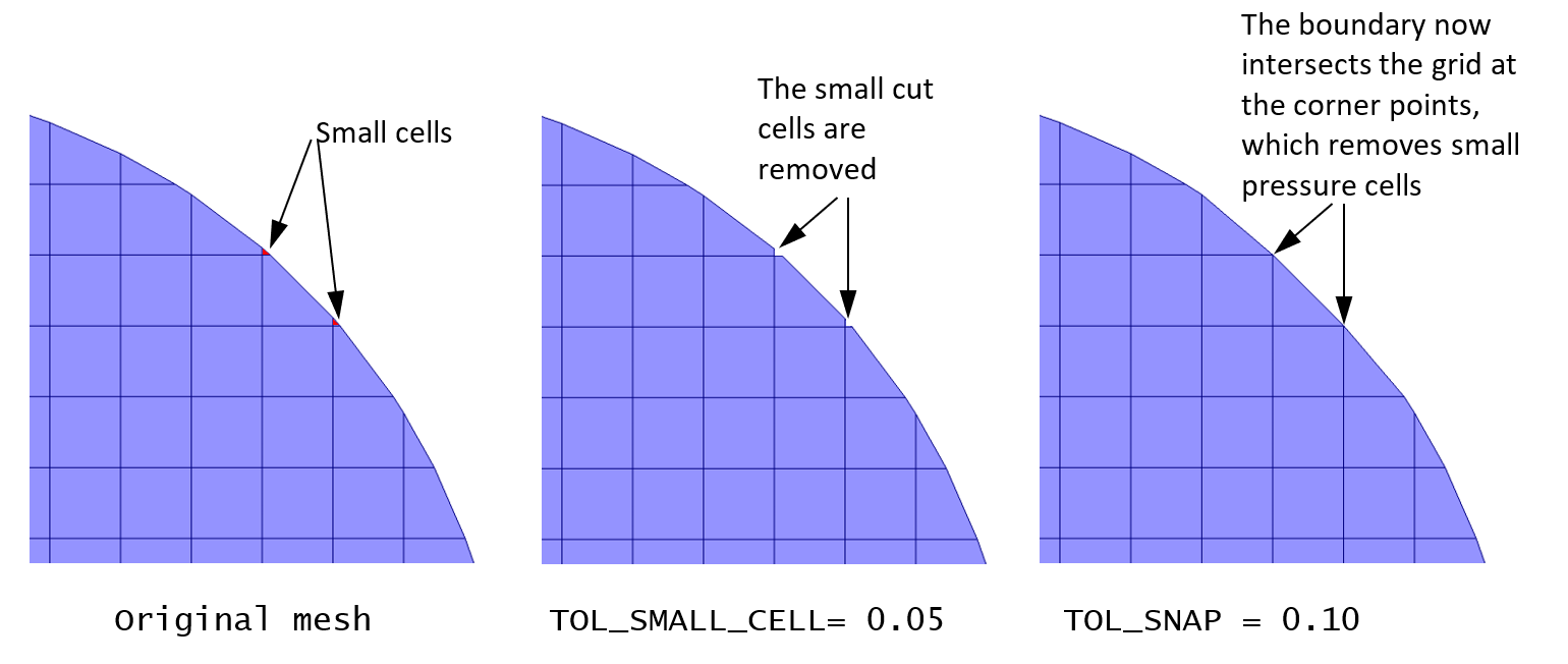
Fig. 12.1 Removing small cut-cells¶
12.6. Discrete Element Model (DEM)¶
12.6.1. How to provide initial particle positions in particle_input.dat file?¶
We can read the initial particle data from a text file, called particle_input.dat.
The format of this file has changed in the 20.3 release. The old file version can still
be used but it is recommended to use the latest format.
To use the file rather than the automatic particle generation (i.e. from Initial Conditions regions), go to the Solids > DEM pane, and leave the “Enable automatic particle generation” checkbox unchecked. Enter a positive number of particles to be read in the “Data file particle count”.
Version 2.0 (MFiX 20.3 release)
The new format allows to either read variables or set a constant value for all particles. The file contains a long header where information about the data is specified. This controls how many columns and which variables are read from the file. Next, the data section contains the data for each particle. Each column corresponds to a variable. In 3D, the first 3 columns are always the x,y and z coordinates of the particle’s center. In 2D, the first 2 columns are always the x,y coordinates of the particle’s center. There are two options for the other variables: either read the data for each particle in the next column, or assign a constant value to all particles.
Below is an example of a particle_input.dat file (the line number is shown on the left and it
not part of the data itself):
Line 1 : File version. Do not change this line.
Lines 2-18 : Instructions to use the file.
Line 19 : This is a 3D geometry. The first 3 columns in the data section will be x,y,z.
Line 20 : We will read data for 35361 particles.
Line 24 : We always read coordinates in the first 2 or 3 columns (do not change)
Line 25 : We do not read particle’s phase ID for each particle. It is assigned a constant value: 1
Line 26 : We will read the particle’s diameter in the next column (column#4).
Line 27 : We do not read particle’s density. It is assigned a constant value: 2500.0 kg/m^3
Line 25 : We do not read particle’s velocity. It is assigned a constant value: (u,v,w) = (0.0,0.0,0.0) m/s
Lines 29-30: This is a cold, non reacting case, we do not read Temperature or species.
Line 31 : We do not have user scalars, so we do not read them.
Lines 32-34: Data header
The data starts on Line 35. Based on the above settings, we need to read, x,y,z, and the diameter of each particles, i.e., 4 columns, for 35361 particles. Only the first few lines of the data is shown.
1 Version 2.0
2 ========================================================================
3 Instructions:
4 Dimension: Enter "2" for 2D, "3" for 3D (Integer)
5 Particles: Number of particles to read from this file (Integer)
6 For each variable, enter whether it will be read from the file
7 ("T" to be read (True), "F" to not be read (False)). When not read, enter the
8 default values assign to all particles.
9 Coordinates are always read (X,Y in 2D, X,Y,Z in 3D)
10 Phase_ID, Diameter, Density, Temperature are scalars
11 Velocity requires U,V in 2D, U,V,W in 3D
12 Temperature is only read/set if the energy equation is solved
13 Species are only read/set if the species equations are solved, and requires
14 all species to be set (if phase 1 has 2 species and phase 2 has 4 species,
15 all particles must have 4 entries, even phase 1 particles (pad list with zeros)
16 User scalars need DES_USR_VAR_SIZE values
17 Data starts at line 35. Each column correspond to a variable.
18 ========================================================================
19 Dimension:    3
20 Particles:    35361
21 ========================================================================
22 Variable      Read(T/F)     Default value (when Read=F)
23 ========================================================================
24 Coordinates:     T          Must always be T
25 Phase_ID:        F          1
26 Diameter:        T
27 Density:         F          2500.0
28 Velocity:        F          0.0 0.0 0.0
29 Temperature:     T          (Ignored if energy eq. is not solved)
30 Species:         T          (Ignored if species eq. are not solved)
31 User_Scalar:     T          (Ignored if no user scalars are defined)
32 ========================================================================
33     X (m)           Y (m)           Z (m)       Diameter (m)
34 ========================================================================
35 -5.07749E-02    -7.98147E-01    -2.00612E-01    9.71052E-03
36 -4.86164E-02    -8.16202E-01    -2.25035E-01    8.34185E-03
37 -3.16460E-02    -8.13702E-01    -2.19164E-01    1.09747E-02
38 -3.32833E-02    -8.25178E-01    -2.19393E-01    9.67983E-03
39 -2.48844E-02    -8.30159E-01    -2.16423E-01    9.84182E-03
40 -8.57591E-03    -8.38121E-01    -2.08773E-01    9.92759E-03
41 -2.75312E-03    -8.32665E-01    -2.00770E-01    1.07560E-02
42 1.57276E-02     -8.37839E-01    -2.08196E-01    1.04387E-02
43 1.96605E-02     -8.31447E-01    -2.15105E-01    9.97808E-03
44 2.71083E-02     -8.26450E-01    -2.19492E-01    9.99619E-03
45 3.55440E-02     -8.28885E-01    -2.15687E-01    9.15771E-03
46 4.45244E-02     -8.28239E-01    -2.11771E-01    1.05089E-02
47 4.70488E-02     -8.22092E-01    -2.19129E-01    9.33350E-03
The particle_input.dat file can be edited in any text editor, including the GUI editor, and be
saved in the project directory. Please run the 2D DEM fluid bed with central jet tutorial from the GUI, or see the DEM initial conditions last section for an example.
Version 1.0 (Prior to MFiX 20.3 release)
The file stores each particle position, radius, density, and velocity. For 2D geometries, it contains 6 columns: x , y, radius, density, u, v. In 3D, it contains 8 columns: x , y, z, radius, density, u, v, w. The number of lines correspond to the number of particles read, and should match the “Data file particle count” defined in the Solids > DEM tab. The check box “Enable automatic particle generation” must be left unchecked.
Below is an example of a 2D particle_input.dat (only 4 particles shown):
0.2000D-03  0.2000D-03  0.5000D-04  0.1800D+04  0.0000D+00  0.0000D+00
0.6000D-03  0.2000D-03  0.5000D-04  0.1800D+04  0.0000D+00  0.0000D+00
0.1000D-02  0.2000D-03  0.5000D-04  0.1800D+04  0.0000D+00  0.0000D+00
0.1400D-02  0.2000D-03  0.5000D-04  0.1800D+04  0.0000D+00  0.0000D+00
Below is an example of a 3D particle_input.dat (only 4 particles shown):
0.2000D-03  0.2000D-03  0.1000D-01  0.5000D-04  0.1800D+04  0.0000D+00  0.0000D+00  0.0000D+00
0.6000D-03  0.2000D-03  0.1000D-01  0.5000D-04  0.1800D+04  0.0000D+00  0.0000D+00  0.0000D+00
0.1000D-02  0.2000D-03  0.1000D-01  0.5000D-04  0.1800D+04  0.0000D+00  0.0000D+00  0.0000D+00
0.1400D-02  0.2000D-03  0.1000D-01  0.5000D-04  0.1800D+04  0.0000D+00  0.0000D+00  0.0000D+00
12.6.2. How to avoid particles going through solid walls in DEM simulations?¶
This is a common issue that arises when particles are too soft. Increasing the spring stiffness (kn and kn_w) typically helps resolve the issue.
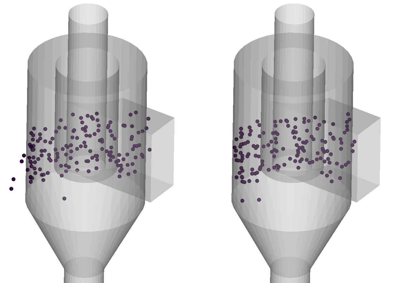
Fig. 12.2 Left: Soft particles (kn=kn_w=100 N/m) going through the cyclone wall. Right: Harder particles (kn=kn_w=1000 N/m) bouncing off the wall.¶
The spring stiffness can be adjusted in the Solids>DEM pane:
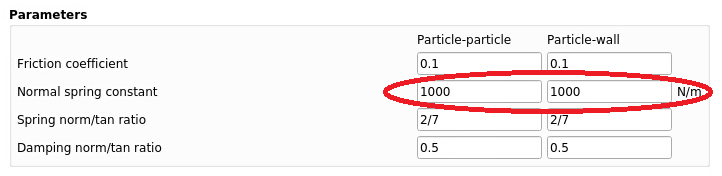
Fig. 12.3 Spring stiffness settings in the GUI¶
Other possible reasons DEM particles may go through the wall:
Missing facets from the STL files: If the STL file is not waterproof, particles can go through the holes. The STL file must be inspected and corrected to fix this issue. The STL file should also not have facets with an angle smaller than the facet angle tolerance (Mesh> mesher pane).
DEM solids time step is too large. If the DEM solids time step is too large, collisions may be missed and particles can go through the wall. Increasing the spring stiffness will automatically reduce the solids time step, but it may be necessary to increase the DEM time step factor (Solids>DEM pane). It is recommended to not lower the DEM time step factor below the default value of 50.
12.7. SuperQuadric Particle Model (SQP)¶
12.7.1. How to specify the particle shape?¶
The shape of non-spherical particles is defined with five parameters, \(a, b, c, m, n\). The surface of the particle is defined with the following superquadric equation:
The exponents m and n in the superquadric equation above correspond to \(\epsilon_1 = \frac{2}{n}\) and \(\epsilon_2 = \frac{2}{m}\) in references [1-3]. The notation used in MFiX is consistent with [4].
The use of exponents m and n allows for a more efficient evaluation of the superquadric equation. There are combinations of m and n values that make the exponent functions much faster in various computations of the superquadric surface equation and its derivatives. The speedup is considerable for favorable values compared with non-favorable values (6-fold speedup in the exponent computation itself). This can translate to an overall speedup of up to 5 for granular flow and up to 2 for gas/solids flows (actual speedup will vary). It is recommended to select these favorable combinations of m and n. [Mathematical details: since the exponents ‘m’, ‘n’ and ‘n/m’ appear in the fundamental equation for superquadrics, these powers are evaluated frequently, so if they are integers, or quarter-integers, the powers can be evaluated efficiently using multiplication and square roots. General floating-point exponentiation is quite slow by comparison.]
To help specify the superquadric parameters, it is recommended to use the superquadric designer (Solids> Material pane). A new interactive widget will pop up, where a, b, c, m and n can be specified. The particle shape can be previewed and the bounding sphere diameter will be automatically calculated.
When the “Constrain exponents to favorable values” is checked, values of m and n will snap to the closest favorable combination. Please note that changing m can also change the value of n since they are linked to form a favorable combination. The list of favorable combination can be seen in the exponent map. Click on “show exponent map” to view the map. The map is interactive, clicking on or near a dot in the map will select a favorable combination.
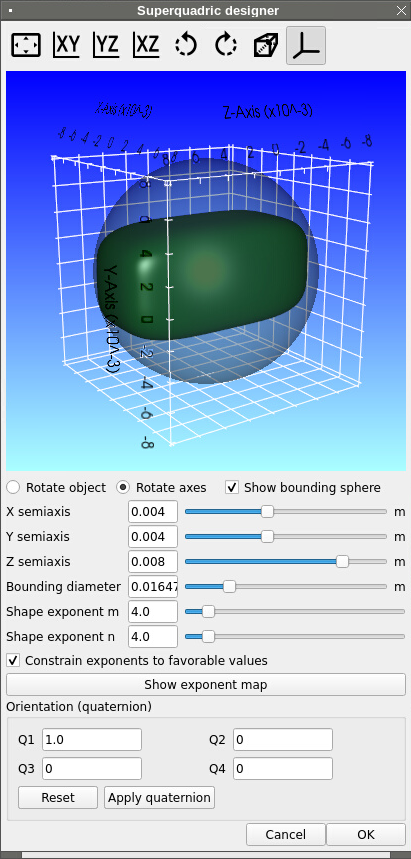
Fig. 12.4 Superquadric designer¶
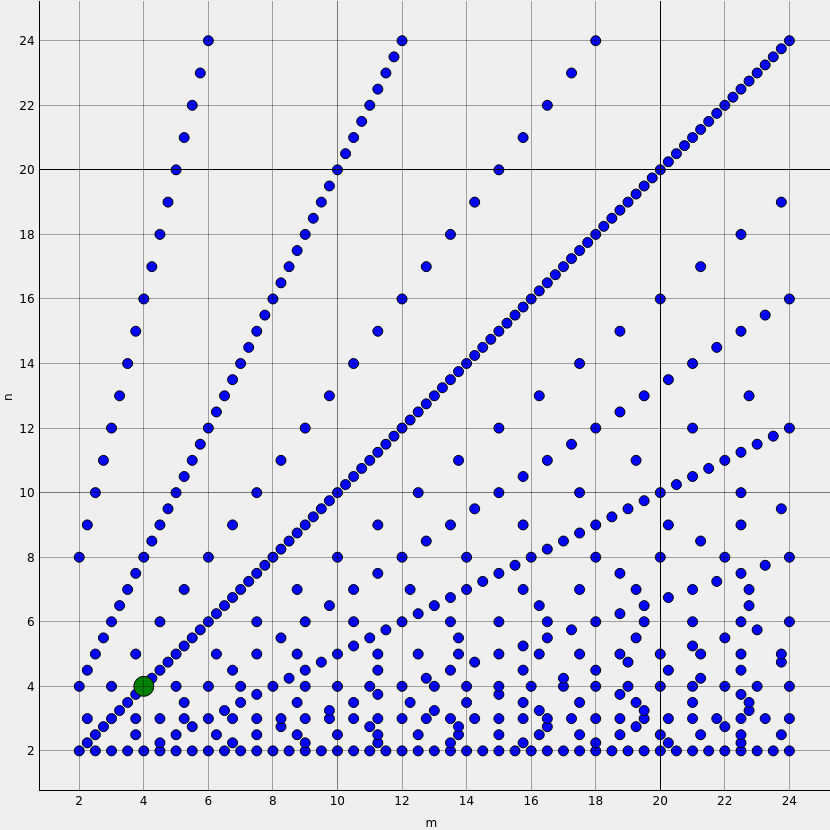
Fig. 12.5 Favorable exponent map¶
[1] Gao, X. Y., J.; Portal, R. J. F.; Dietiker, J. F.; Shahnam, M.; Rogers, W. A. “Development and validation of SuperDEM for non-spherical particulate systems using a superquadric particle method,” Particuology Vol. 61, 2022, pp. 74-90. https://doi.org/10.1016/j.partic.2020.11.007
[2] Gao, X. Y., Jia; Lu, Liqiang; Li, Cheng; Rogers, William A. “Development and validation of SuperDEM-CFD coupled model for simulating non-spherical particles hydrodynamics in fluidized beds,” Chemical Engineering Journal Vol. 420, 2021, p. 127654. https://doi.org/10.1016/j.cej.2020.127654
[3] Gao, X. Y., J.; Lu, L. Q.; Rogers, W. A. “Coupling particle scale model and SuperDEM-CFD for multiscale simulation of biomass pyrolysis in a packed bed pyrolyzer,” Aiche Journal Vol. 67, No. 4, 2021, p. 15. https://doi.org/10.1002/aic.17139
[4] Becker, Verena & Birkholz, Oleg & Gan, Yixiang & Kamlah, Marc. (2021). Modeling the Influence of Particle Shape on Mechanical Compression and Effective Transport Properties in Granular Lithium-Ion Battery Electrodes. Energy Technology. 9. https://doi.org/10.1002/ente.202000886
Examples:
a |
b |
c |
m |
n |
shape |
view |
|---|---|---|---|---|---|---|
0.003 |
0.003 |
0.003 |
2.0 |
2.0 |
sphere |
|
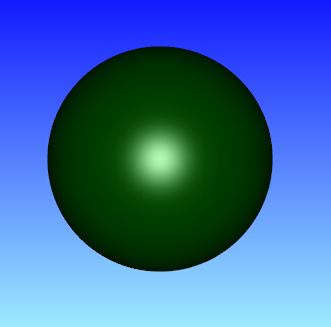
0.003 |
0.001 |
0.006 |
2.0 |
2.0 |
ellipsoid |
|
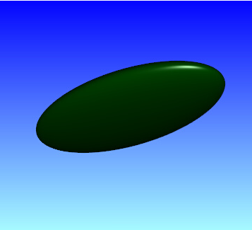
0.003 |
0.001 |
0.006 |
8.0 |
8.0 |
cuboid |
|
0.003 |
0.003 |
0.006 |
2.0 |
8.0 |
cylinder |
|
12.7.2. Recommended settings¶
When running the SQP solver, it is recommended to use the Hertzian collision model with large values of the Youngs modulus (larger than 1.0E7 Pa) to avoid excessive overlap. For gas/solids flows, the interpolation scheme should be set to ‘DPVM_SATELLITE’.
12.8. Meshing¶
12.8.1. How to verify/flip STL file facet normals?¶
When using an STL file to define the geometry, a normal vector is associated with each facet (triangle). The direction in which the normal vector points indicates the fluid region. It is important to verify the normal vectors points in the desired direction before running the simulation.
To show the normal vectors in the Model view, expand the geometry view settings on the right and check “Show Normals”. It may be necessary to adjust the scale to get a better view. The figure below shows an example of a cylinder with vectors pointing towards the interior region of the cylinder. This will correspond with an internal flow simulation where the fluid region is located inside the cylinder and the outside region is not part of the simulation.
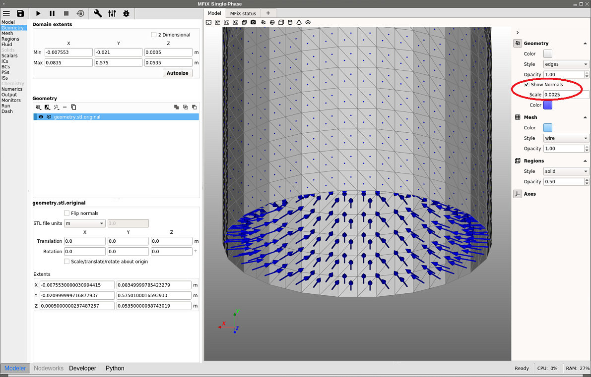
Fig. 12.6 Displaying STL normals, internal flow¶
If the normal vectors are not pointing in the correct direction, the normals can be flipped by checking the “Flip normal” box for any selected stl file. To model an external flow using the same geometry as above, flip the normals and the change will be reflected in the Model view (see figure below). Now the normals points towards the outside of the cylinder, and the region inside the cylinder will not be part of the computation.
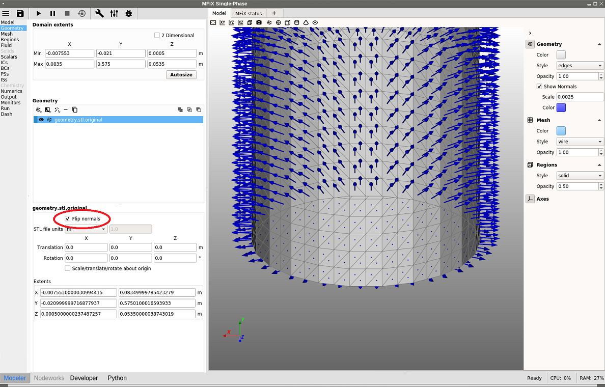
Fig. 12.7 Flipping STL normals to model an external flow¶
12.8.2. How to manually specify a grid partition for DMP runs?¶
When running a simulation in parallel (DMP) mode, the parallel decomposition is by default uniform in each direction and the number of partitions is set by NODESI, NODESJ, and NODESK in the x,y and z directions, respectively. The default partition may not always be the most efficient. For example, a DEM simulation of a fluidized bed where most particles are at the bottom of the bed may run faster if smaller partitions are set at the bottom, where many particles are located and a large partition is used in the freeboard. This will better distribute particles among processors, and provide a better load balance.
Let’s assume the mesh contains 20x100x20 cells (IMAX=20, JMAX=100, KMAX=20) and we use 16 cores with a 2x4x2 partition (NODESI=2, NODESJ=4, NODESK=2). Assume particles are roughly located within the bottom half of the bed throughout the simulation. With the default (uniform) decomposition, each vertical partition will contain JMAX/NODESJ=25 cells (Figure 8.6). This means 8 cores will remain mostly idle with respect to particle tracking and collision.
Instead, we can distribute cells in the y-direction so that the vertical partitions have roughly the same number of particles. This can be achieved with 10, 10, 10, and 70 cells from bottom to top. (Figure 8.7).
Due to the symmetry of the problem in x and z directions, no adjustment is needed in these directions, and a uniform distribution is adequate.
Note that the custom partition will provide better load balance for particles but will make the fluid calculation slower since fluid cells will be unbalanced. However, since a large majority of the time is spent in the DEM loop, it should be beneficial to customize the partition.
To specify this decomposition, the following gridmap.dat needs to be saved in the project directory:
The first line specifies the values of NODESI, NODESJ, NODESK.
2 4 2 ! NODESI, NODESJ, NODESK
The next two lines (NODESI=2) specify the partition sizes in the x-direction. Here each partition contains 10 cells:
0        10
1        10
The next four lines (NODESJ=4) specify the partition sizes in the y-direction. Here three partitions at the bottom contains 10 cells each, and the last partition contains 70 cells:
0        10
1        10
2        10
3        70
The last two lines (NODESK=2) specify the partition sizes in the z-direction. Here each partition contains 10 cells:
0        10
1        10
Below is the entire gridmap.dat file:
2        4          2    ! NODESI, NODESJ, NODESK
0        10
1        10
0        10
1        10
2        10
3        70
0        10
1        10
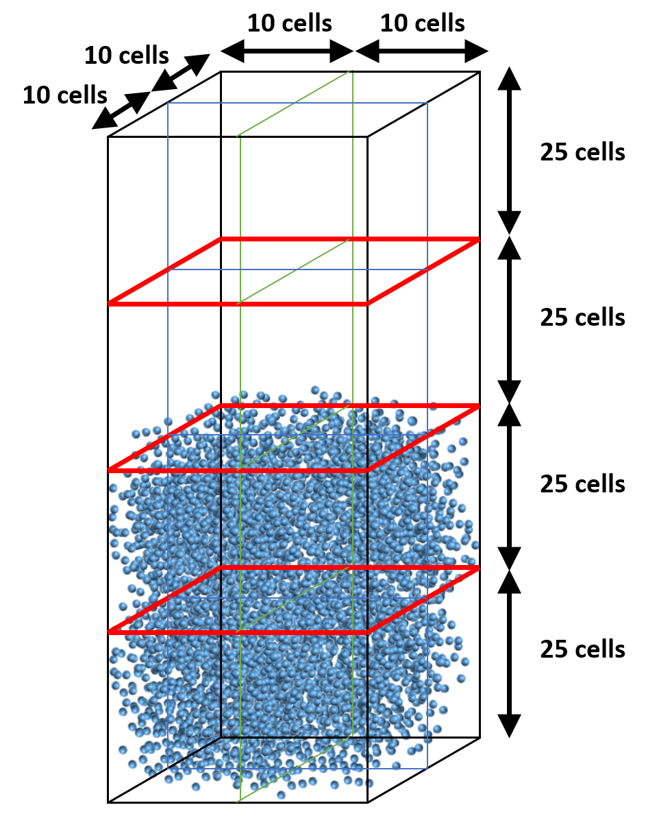
Fig. 12.8 Default partition (uniform distribution)¶
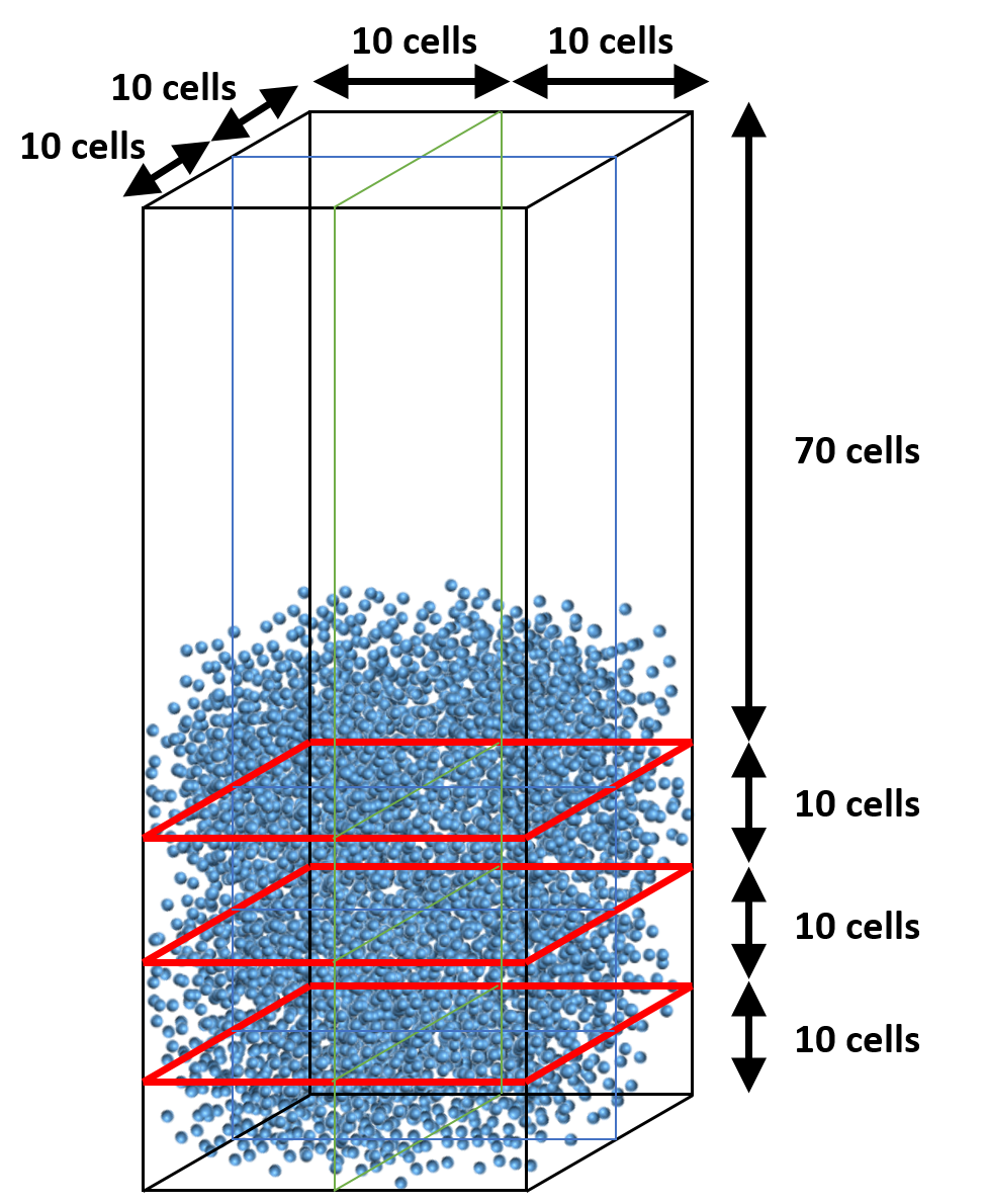
Fig. 12.9 Adjusted partition in vertical direction (specified with gridmap.dat)¶
12.9. Particle in Cell (PIC)¶
12.9.1. How To Choose a Good Statistical Weight for PIC Runs?¶
One key to creating efficient and accurate particle in cell (PIC) simulations is choosing an appropriate value for the statistical weight of particles per parcel. The user needs to balance desired solids weight fraction, mesh density and solids mass error with computational speed and physics.
The PIC statistical weight in MFIX (IC_PIC_CONST_STATWT or BC_PIC_CONST_STATWT) represents how many particles are represented by each parcel. The parcels themselves must be of discrete number in a simulation, but because statistical weight is a math construct, partial particles may occur mathematically.
To facilitate statistical weight selection, it is desirable to create a spreadsheet that illustrates how its selection can impact simulation conditions, or the following logic may be prescribed.
Collect the following information:
Diameter of an equivalent single spherical particle (m)
Mass density of particles (kg/m 3 )
Max-pack solids fraction of particles for simulation
Choose a mesh for the simulation. Separately, calculate an average cell volume (m 3 ) and a minimum cell volume (m 3 ).
Using max-pack solids fraction (which must be defined for PIC, 1-EP_STAR), calculate an average cellular volume available for solid (m 3) and a minimum cellular volume available for solid (m 3).
Using particle diameter, calculate the number of spherical particles these average cellular volumes available for solid represent. Assuming a uniform mesh, this calculated number, as a rounded-down integer, would represent the maximum statistical weight one can choose in a PIC simulation, although it is highly unlikely one would choose this value. In a variable mesh, the value associated with the minimum cell volume is the maximum statistical weight. (Note: using an average cellular volume for this calculation allows a balance of parcel load in both large and small cells.) Note that a user does not need to know the solids fraction distribution that they expect in a simulation, only the max-pack solids fraction, which is a constant.
Now the balancing act between parcel count, actual solids fraction and mass error begins. First, choose a statistical weight value. An easy way to make a first approximation is to use the maximum statistical weight from (4) and divide by an integer which in your mind represents the number of parcels you want per cell. Statistical weights derived like this will naturally give a solids fraction very close to whatever the original desired value from (1) was, and minimize mass error in a simulation. The statistical weight does not need to be an integer, because partial particles make sense in PIC. While the parcel count in an individual cell will initially begin as an integer, there is no limitation that says an integer number of particles must make up a parcel. Choosing an integer value for statistical weight does make it simple to imagine the parcels as grouped entities of particles, but it may interfere with expectations for representative solids volume fraction per cell. Note, however, that regardless of what the user specifies as a statistical weight, the MFIX program will collect truncated mass values in each cell until enough mass to represent a full parcel accumulates, whereupon a single extra parcel will be placed in the domain.
It is advisable to inspect your fully populated PIC parcel domain to make sure you have not applied a value that does not make visual or physical sense. This is particularly true for very dilute flow and highly packed flow. For dilute flows, choosing a statistical weight that is too large will result in a simulation that cannot possibly capture expected flow dynamics. In a highly packed flow, choosing a statistical weight that is too low may result in non-physical packing, and an overly large local solids fraction. As such, be certain to note the values reported in the MFIX output for desired solids fraction and calculated solids fraction, then assure yourself that the numbers are within some reasonable error band.
12.9.2. PIC statistical weight example¶
During initialization, the user can choose any region to fill with parcels. If a distinct mass of particles is needed in a region at start-up, the user must pre-conceive an appropriate volume of cells and associated solids fraction to achieve that mass.
For example, if a user wants :
0.1 kg of 0.001 m particles with density 1000 kg/m 3
in a volume that is 0.1 x 0.1 x 0.1 m 3 defined by a 10 x 10 x 10 mesh
with max-pack of 0.4 (theoretical limit of random packing of spheres is 0.36)
First, calculate the volume of 1 particle: V_particle= \(\pi\)/6 (0.001)3 = 5.236E-10 m 3
Calculate the mass of 1 particle: m_particle=(1000 kg/m 3 )(5.236E-10 m 3) = 5.236E-7 kg
Calculate single cellular volume: V_cell=(0.1m) 3/((10×10×10))=1.0E-6 m 3
Calculate available volume for parcels: (1-0.4)( 1.0E-6 m 3) = 6.0E-7 m 3
For simplicity, we assume that the particles are evenly distributed among the 1000 cells. That means, each cell needs 0.100 kg/1000cells = 0.0001 kg of solid. In turn, that means each cell needs 0.0001 kg / 5.236E-7 kg = 190.985 particles. From this particle loading, you can choose a statistical weight based on the number of particles. For example, you could choose 190.985 as the statistical weight and get 1 big parcel (unwise), or you could choose, say, a statistical weight of 10 and get 19 parcels with a small local mass error. The small errors are accumulated, and when large enough, an extra parcel will be placed locally in the mesh to account for the local loss. Note that if the user does not want to fill an initial area at maximum packing, simply choose a different value for solids fraction and recalculate. Having a preconception of how “loose” a particle bed should be is very helpful for reducing the transient in a simulation start-up.
Likewise, if a mass inflow boundary is prescribed in the PIC model, a similar logic must be followed. The key is to make sure that the statistical weight used for the boundary flow condition is reasonable (as in, the number of particles per parcel will fit into the cell(s) that abut the boundary condition specification). MFIX will control the mass itself by accounting individual particle mass and randomly assigning parcels through the BC window. Note that smaller statistical weights produce less local mass error, but the user must choose their own balance between statistical weight and computational speed.
12.9.3. Meshing Basics for PIC Runs¶
There are three common mistakes a user may make when setting up a PIC run. The first represents a misunderstanding of MFIX-PIC which is necessarily a 3-D model. That means, you cannot specify a 2-D simulation with MFIX-PIC. Second, the interpolation algorithm which undergirds the MFIX-PIC model requires a minimum of 3-cells in each direction through a geometry to give a robust solution. It is important to check small geometric regions of the mesh that might pass through an orifice or channel to assure that there are at least 3 cells available for calculations to work in a hydrodynamically stable way. Smaller cell distributions will not crash the model, but you may get unexpected flow behavior. Finally, choosing statistical weights that in comparison to mesh give less than one parcel per mesh cell will give errant solutions. (See section on choosing good statistical weights.) Note that one of the benefits of PIC is that it allows for a somewhat coarse mesh with a large particle count, but a user needs to balance mesh and parcel count in a reasonable way.
12.9.4. Choosing Primary PIC Parameters¶
PIC parcels do not behave like DEM particles. There are no Newtonian physical laws that govern collisions. Instead, PIC utilizes a solids stress ( \(\tau_p\)) field that influences solids motion through a coupling with the momentum equation. Specifically, the solids stress is calculated as:
\(\tau_p=\frac{P_p \epsilon_p^\gamma}{\max[\epsilon_{cp} - \epsilon_p , \delta(1-\epsilon_p)]}\)
In MFIX, the parameters that the user can control to define this solids stress are an empirical pressure constant (PSFAC_FRIC_PIC ( \(P_p\) ), a volume fraction exponential scale factor (FRIC_EXP_PIC ( \(\gamma\)), void fraction at maximal close packing(EP_STAR ( \(\epsilon_{cp}\)) and a non-singularity constant (FRIC_NON_SING_FAC ( \(\delta\)). The only other variable at play within the solids stress model is solids void fraction ( \(\epsilon_p\) ) which is calculated dynamically as the simulation progresses.
The parameters used in PIC are very robust. The default values of \(P_p\) =100, \(\gamma\) =3, \(\delta\) =1.0E-7 should work well for most systems. There should be no reason to change \(\delta\). The value for \(\epsilon_{cp}\) will vary depending on your application, although it is worth noting that there is a theoretical limit of ~0.36 for the random packing of equal spheres. It is important to note that \(\epsilon_{cp}\) represents the void or gas fraction per cell, and not the solids fraction. The effects of changing the values of \(P_p\) and \(\gamma\) are very problem specific. For example, sedimentation cases (on which the solids model was originally built) will model best with \(P_p\) =1, \(\gamma\) =2 so that gravity has the most effect on the system through the momentum equation. But, very dynamic cases (U_mf>10) where we expect the solids to more greatly affect the hydrodynamics of the system may respond better with selections like \(P_p\) =1000, \(\gamma\) =3. Essentially, like all CFD models, it may be necessary to tune the PIC model to your specific case. As a rule of thumb, larger \(P_p\) at constant \(\gamma\) will result in particles that move more dynamically (as the selection will linearly increase the solids stress). But, larger \(\gamma\) at constant \(P_p\) will reduce the solids stress exponentially and dampen overall solids motion. The largest values of solid stress will occur when \(P_p\) is large and \(\gamma\) is small.
12.9.5. Choosing Secondary PIC parameters¶
Like DEM, the user can control restitution factors that affect parcel motion. MPPIC_COEFF_EN_WALL applies a scale factor to the normal component of velocity after a parcel interacts with a wall. Likewise, MPPIC_COEFF_ET_WALL applies a scale factor to the tangential components of velocity after a parcel interacts with a wall. There are two other empirical factors available in MFIX-PIC. The first is MPPIC_COEFF_EN1 which is an overall scale factor that can dampen the effect of the entire solids stress model, and MPPIC_VELFAC_COEFF which is a scale factor that effects the value of bulk solids velocity through an evaluation of gas-solids slip velocity. These last two factors should remain at default values unless you are working as an advanced user and understand the open source PIC code implicitly.
PIC Collision Damping —-====————-
An empirical collision damping feature has been added to the MFIX-PIC model. The feature includes a calculation for collision frequency based on statistical likelihood. From this frequency, a small change in velocity is calculated and applied to parcels locally. The effect is an overall damping of solids velocity, particularly in areas where dense particle flow is apparent. To invoke the feature, the user must select “Collision Damping” in the GUI (Solids>PIC pane) or set the keyword is PIC_COLLISION_DAMPING=.TRUE. in the .mfx file.
12.9.6. Why can’t I define parcels per cell instead of particles per parcel?¶
When creating the MFIX-PIC model, programmers chose to define particles per parcel for two reasons.
The user has full control over the statistical weights of the PIC parcels and is not reliant on the computer code to calculate those values without knowledge of the simulation being run.
In most CFD simulations, mesh can be highly variable. When a user defines parcels/cell, the smallest cell will limit the number of parcels that can be placed in any cell at initialization. By defining particles/parcel, the check we suggest for examining the smallest cell only limits the overall size of the parcel, and a more even solids void fraction can be achieved at start-up. An argument can be made that multiple initialization regions can be created to smooth solids void fraction using the parcel/cell method, but this only complicates set-up.
12.9.7. What is a good number (or range) for the number of parcels per cells?¶
It depends on the kind of simulation you are trying to run, how many processors you have available to you, and what kind of fidelity you expect. Avoid going below 3 parcels/cell in a serial run where there is very little dynamic (like settling).
Typically, around 10 parcels/cell works smoothly. If the simulation looks chunky, reduce the number of particles/parcel, thus upping the parcels/cell count.
12.9.8. What solids model parameter values work best for the PIC model when running 2 densities that are roughly 10x different in magnitude?¶
A density difference like this (say 300 kg/m 3 and 3,000 kg/m 3) will cause natural physical separation in most systems. To capture the best physics in a PIC model where density drives strong gravitational effects, choose \(P_p\) =1 and \(\gamma\) =5 to begin. You may still need to adjust these parameters but these choices will give you a good place to start.