3.11. Hydrogen oxidation in a batch reactor using CHEMKIN mechanism
This tutorial shows how to import thermodynamic information of species and kinetic mechanism from CHEMKIN into MFiX. A batch reactor in a single cell is simulated in this tutorial. The mechanism for the oxidiation of hydrogen from Conaire et al. [1] is applied.
3.11.1. Load the project into MFiX
The basic model has been set up in the input file, “hydrogen_oxidation.mfx”.
On the main menu select
New project.Open the project
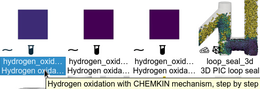
hydrogen oxidation with CHEMKIN mechanism, step by step.
Choose the location for your working directory and click
OK.

Note
The main purpose of this tutorial is to show how to use CHEMKIN mechanism in MFiX. For more details about the model setup, please refer to other tutorials.
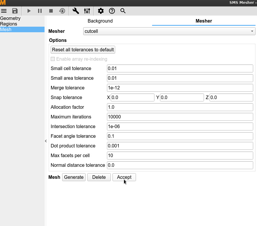
3.11.2. Generate mesh
On the Mesher pane:
Click
Generateto generate the meshClick
Acceptto accept the mesh, and switch to the Modeler tab (bottom left of GUI).
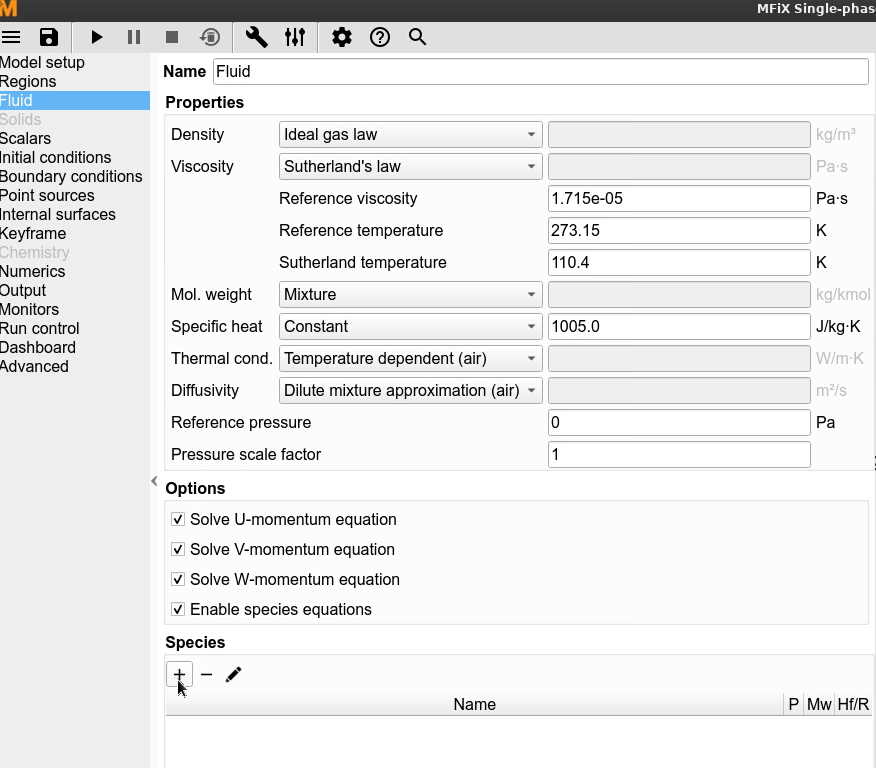
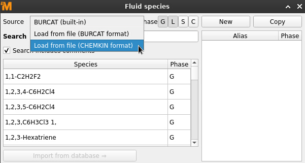
3.11.3. Import species for fluid phase
On the Fluid pane:
Click
 under
under Species. This will open the Fluid species popup window.
Select
Load from file (CHEMKIN format)inSourceof the popup window
Click
Choose file, choose “thermodynamicInfo.txt” in the popup window, and clickOpen.
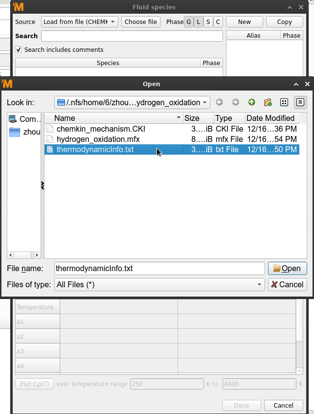
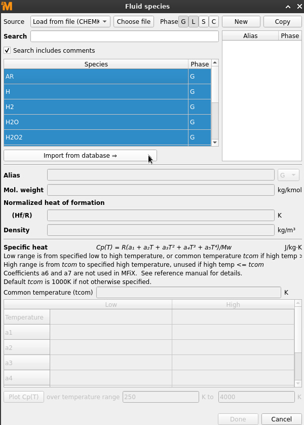
After importing the file, the species defined in the file will show in the window.
Select all the species (click on first species “AR” and drag down) and click
import from databaseto import all species. ClickDone.
Note
Users have the flexibility to select the required species for their case from the provided list. If a species is not defined in the CHEMKIN file, users can import it from the built-in Burcat database or an external Burcat file as well.
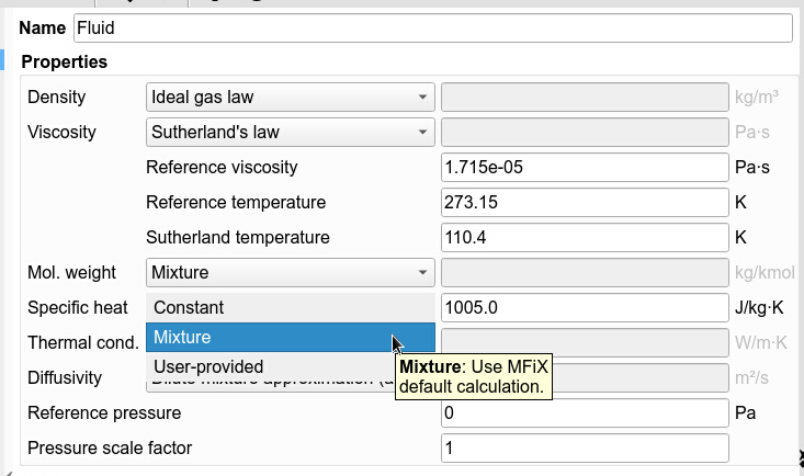
For reacting cases, constant specific heat capacity is not allowed. Change it to “Mixture” in “Properties”.
3.11.4. Create Initial and Boundary conditions
On the Initial conditions pane, set the following conditions as the initial conditions.
Property |
Initial Value |
|---|---|
Volume Fraction |
1.0 |
Temperature |
800 K |
Pressure |
101325 Ps |
U-Velocity |
0.0 m/s |
V-Velocity |
0.0 m/s |
W-Velocity |
0.0 m/s |
Composition |
H2: 0.1, O2: 0.8, N2: 0.1, OH: 0.0, TestSpecies: 0.0 |
On the Boundary conditions pane, No-Slip and adiabatic walls have been setup.
3.11.5. Import kinetic mechanism
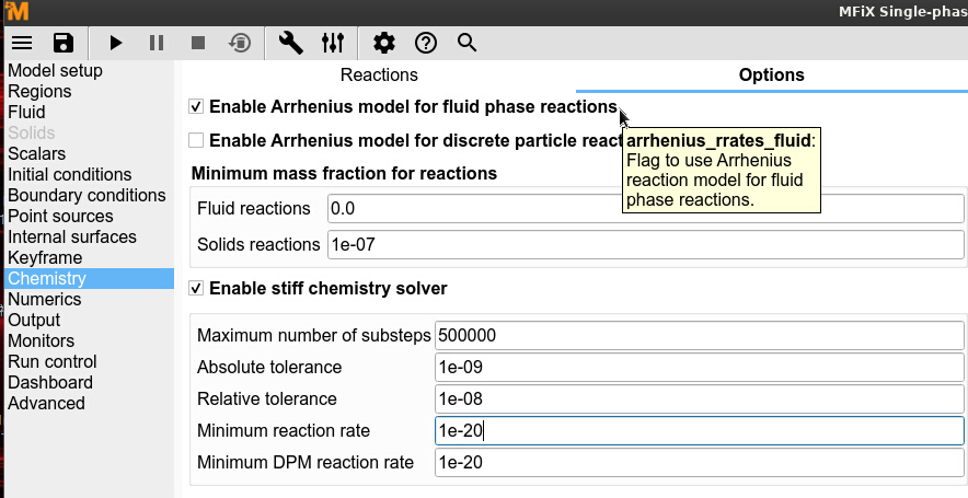
On the Chemistry pane, Options sub-pane:
Check the
Enable Arrhenius model for fluid phase reactionscheckboxChange the
Minimum mass fraction for reactionsforFluid reactionsto 0 to consider all species with mass fraction larger than 0 in the reactionsCheck the
Enable stiff chemistry solvercheckboxChange the
Absolute tolerance,Relative toleranceandMinimum reaction ratein stiff solver to be 1e-09, 1e-08 and 1e-20.
Note
Users can change the minimum mass fraction for reactions and the parameters for stiff solver based on the accuracy requirement of their cases.
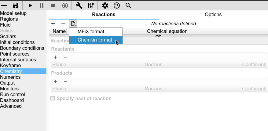
On the Chemistry pane, Reactions sub-pane:
Click

Load reaction definitions from text fileand selectChemkin formatSelect the mechanism file “chemkin_mechanism.CKI” in the popup window. Click
Open.
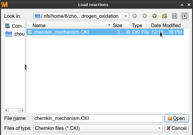
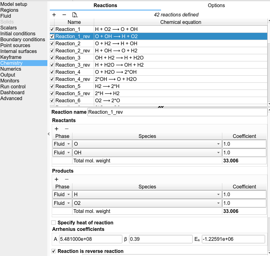
Then all the reactions with all the information will be imported
3.11.6. Setup output, monitor and run parameters
The output, monitor and run parameters have been setup. Users can modify them based on their own requirement.
To check the change of species, we need to save the species into the output/monitor files.
On the Output pane:
Select the
VTKsub-pane. An output has been setup.In the
FluidofSelect cell data to writeat the bottom of GUI, select the checkboxes for species inMass fraction.
On the Monitors pane:
An monitor has been setup with the gas temperature saved every 0.001s.
In the
FluidofSelect cell data to writeat the bottom of GUI, select the checkboxes for species H2 and O2 inMass fraction.
3.11.7. Run the project
Save the project by clicking the
 button
Run the project by clicking the
 button
On the
Run Solverdialog, select the default solver from the combo-boxClick the
Runbutton to start the simulation
3.11.8. View results
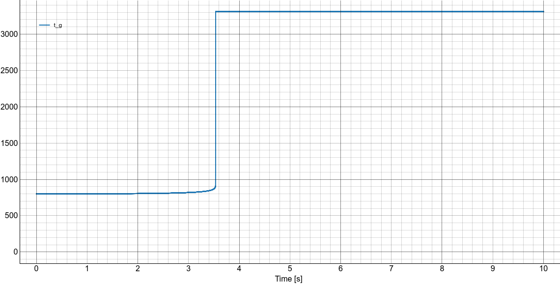
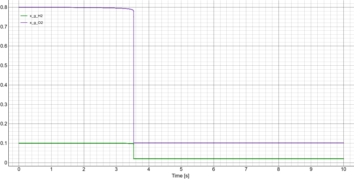
This tutorial simulates the oxidation of H2 in a batch reactor. Users should expect to see consumption of H2 and O2 and a temperature increase from the exothermic reaction.
Results can be viewed, and plotted, while the simulation is running.
Create a new visualization tab by pressing the
next to the Model tabSelect
Monitorsto view the results.On the
Monitorsresults tab, the visibility of the variables can be controlled with the menu under the plot.
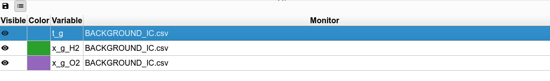
Hide the gas temperature by unclick the
 for variable t_g.
The following plot with the transient changes of the mass fraction of H2 and O2 will be shown.
for variable t_g.
The following plot with the transient changes of the mass fraction of H2 and O2 will be shown.
Hide the gas species by unclick the
for variables x_g_H2 and x_g_O2.
The following plot with the transient change of the gas temperature will be shown.