3.12. Hydrogen oxidation in a batch reactor using transport data in CHEMKIN format

This tutorial shows how to use the transport data in CHEMKIN format for the calculation of gas viscosity, thermal conductivity and diffusivity. The mechanism and transport data for the oxidiation of hydrogen from Conaire et al. [1] are applied.

The project is based on the tutorial for hydrogen oxidation in a batch reaction using CHEMKIN mechanism. The thermodynamic information of species and kinetic mechanism in CHEMKIN format have been imported. For more detailed about how to import these information, please check the above tutorial.

3.12.1. Load the project into MFiX

The basic model has been set up in the input file, “hydrogen_oxidation_transport.mfx”.

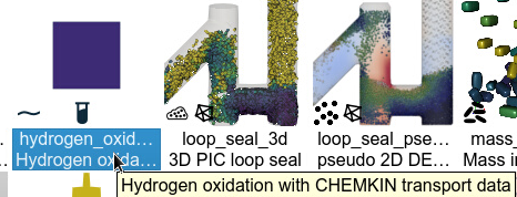
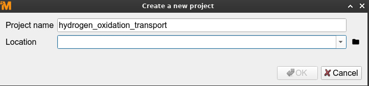
• On the main menu select New project.

• Open the project hydrogen oxidation with CHEMKIN transport data.

• Choose the location for your working directory and click OK.

Note

The main purpose of this tutorial is to show how to use CHEMKIN transport data in MFiX. For more details about the model setup, please refer to other tutorials.

3.12.2. Generate mesh

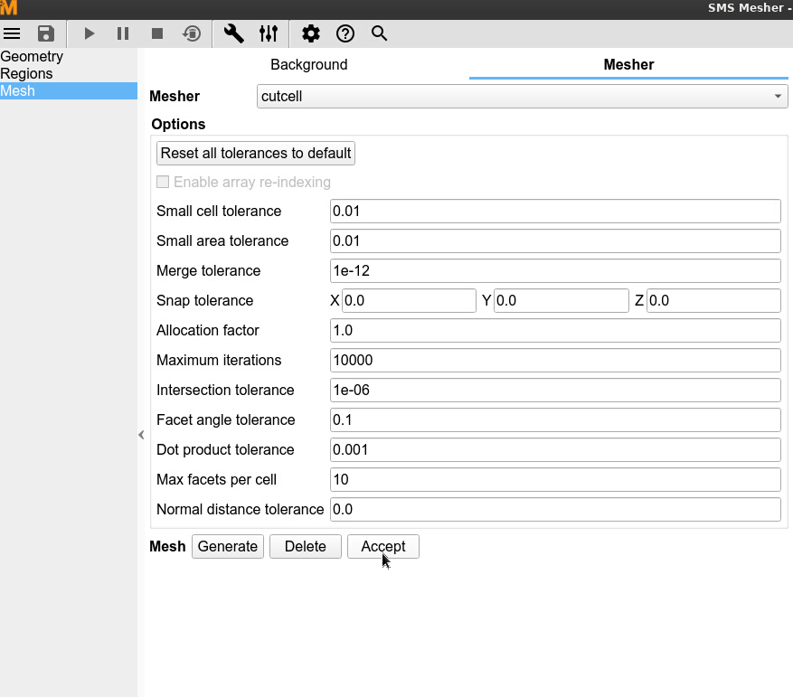
On the Mesher pane:

• Click Generate to generate the mesh

• Click Accept to accept the mesh, and switch to the Modeler tab (bottom left of GUI).

3.12.3. Setting viscosity model for fluid phase

On the Fluid pane:

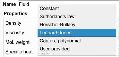
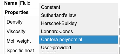
• Click the models for Viscosity. There are six different models. Lennard-Jones and Cantera polynomial will be discussed in this tutorial, which use the transport data.

Note

These two models can only be selected when the species are defined in gas phase.

3.12.3.1. Using Lennard-Jones model for gas viscosity

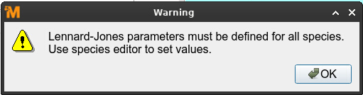
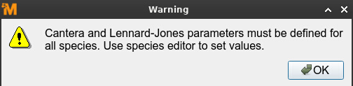
• Select Lennard-Jones for Viscosity. The following warning will popup to remind users adding the required parameters. Click OK.

• Select one of the species in the Species pane. Double click to edit, or click the edit button . The boxes to add the Lennard-Jones parameters are shown in the popup window.

Users have two options to add the Lennard-Jones parameters:

• Add them in the box manually

• Import them from an external file, which has the transport data in CHEMKIN format. In the transport file from CHEMKIN, species name following with its molecular shape, Lennard-Jones potential well depth, Lennard-Jones collision diameter, dipole moment, polarizability and rotational relaxation collision number at 298K are provided.

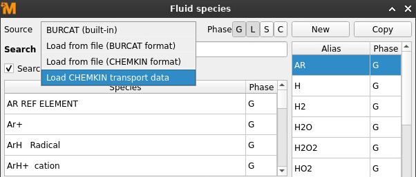
  The following steps show how to import the file for transport data

  • Select Load CHEMKIN transport data in Source of the popup window

  

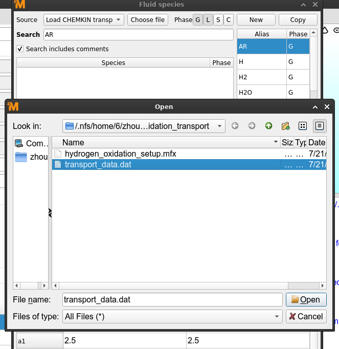
  • Click Choose file, choose “transport_data.dat” in the popup window, and click Open.

  

  • After importing the file, the Lennard-Jones parameters will be added automatically in the corresponding box

  • Click Done to close the popup window and add other settings

Note

Multiple transport files can be imported. The data will be overwritten based on the last imported file if species is defined in multiple files.

3.12.3.2. Using Cantera polynomial model for gas viscosity

• Select Cantera polynomial for Viscosity.

• The following warning may popup to remind users adding the required parameters.

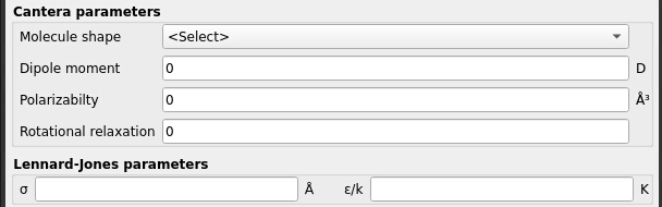
• Select one of the species in the Species pane. Double click to edit, or click the edit button . The boxes to add the transport data for this model are shown in the popup window. The default values of dipole moment, polarizability and rotational relaxation of 0 will be shown.

Similar to Lennard-Jones model, users have two options to add the parameters.

• Add them in the box manually

• Import them from an external file, which has the transport data in CHEMKIN format. Follow the same steps as Lennard-Jones model to import the file.

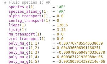
Only the molecular shape, dipole moment, polarizability and rotational relaxation need to be defined. The GUI will automatilcally compute the polynomial coefficients poly_mu_g using Cantera and save them into .mfx file.

3.12.4. Setting thermal conductivity model for fluid phase

On the Fluid pane:

• Click the models for thermal conductivity. There are six different models. Lennard-Jones and Cantera polynomial will be discussed in this tutorial, which use the transport data.

Note

Same as viscosity model, these two models can only be selected when the species are defined in gas phase.

3.12.4.1. Using Lennard-Jones model for gas thermal conductivity

• Select Lennard-Jones for Thermal conductivity with the popup warning to remind users adding the required parameters.

• Select the species in the Species pane. Double click to edit, or click the edit button .

• Add the Lennard-Jones parameters in the popup window by adding them manually or importing an external file.

3.12.4.2. Using Cantera polynomial model for gas thermal conductivity

• Select Cantera polynomial for Thermal conductivity with the popup warning for adding the required parameters.

• Select the species in the Species pane. Double click to edit, or click the edit button .

• Add the required parameters in the popup window by adding them manually or importing an external file.

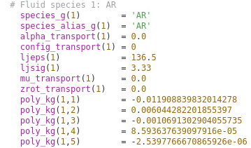
Only the molecular shape, dipole moment, polarizability and rotational relaxation need to be defined. The GUI will automatilcally compute the polynomial coefficients poly_kg using Cantera and save them into .mfx file.

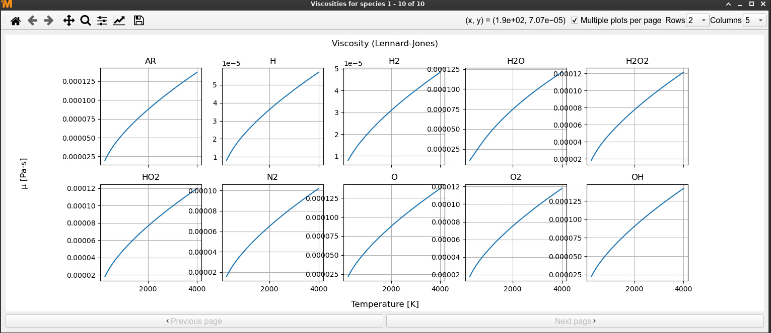
3.12.5. Plotting the viscosity and thermal conductivity of gas species

Users can plot the viscosity or thermal conductivity of each gas species as a function of temperature.

• Select one of the species in the Species pane. Double click to edit, or click the edit button .

• Select thermal conductivty or viscosity for plot at the bottom of the popup window.

• Click Plot to show the figures. Users can changes the number of plots in each page by changing the number of rows and columns at the top-right corner of the plot.

3.12.5.1. Viscosity and thermal conductivity with Lennard-Jones model

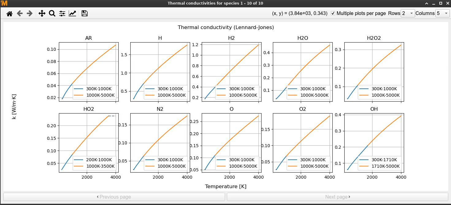
Note

There are two ranges for the thermal conductivity based on the common temperature of species from the thermodynammic data. It is because the thermal conductivity using Lennard-Jones model depends on the heat capacity of species, which has different coefficients at different temperature ranges.

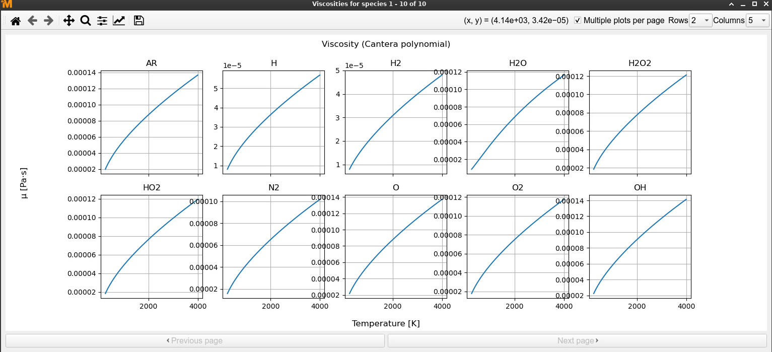
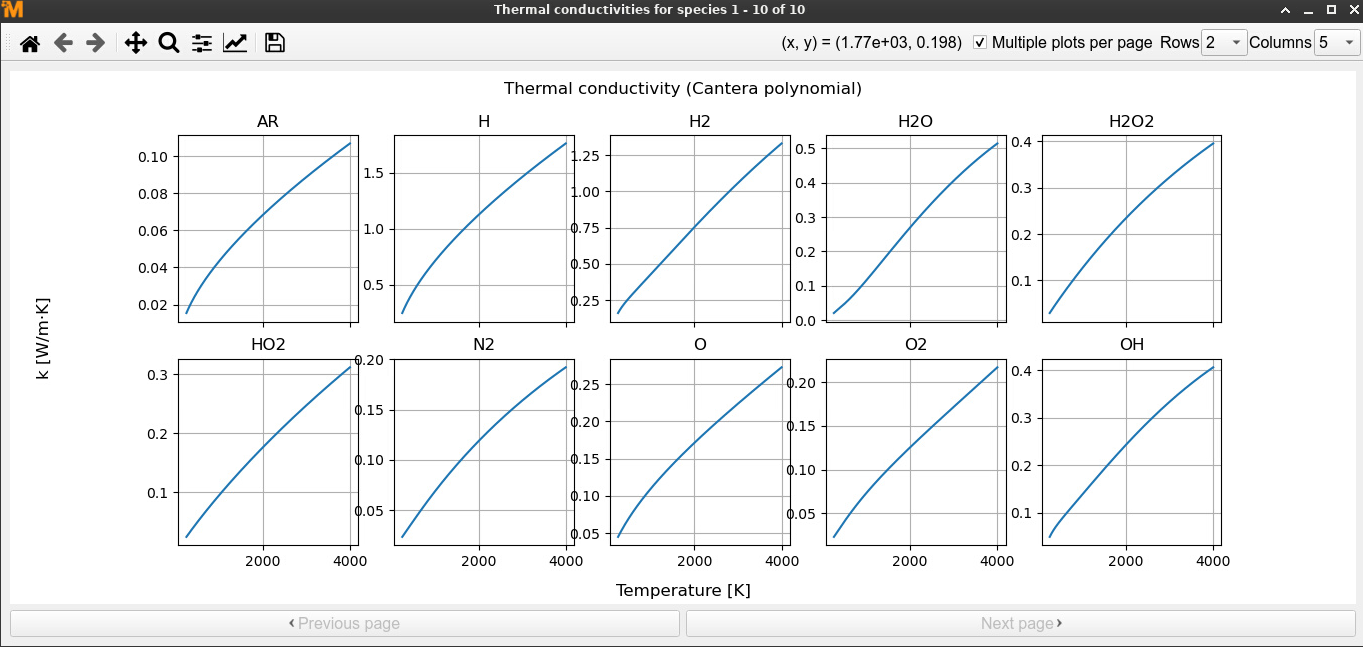
3.12.5.2. Viscosity and thermal conductivity with Cantera polynomial model

3.12.6. Using the transport data for the diffusivity model

The Lennard-Jones parameters can be used for the calculation of diffusivity as well.

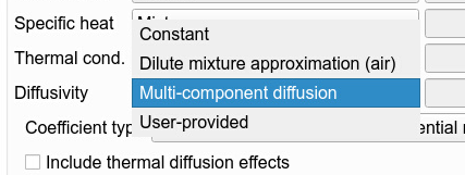
• Select Multi-component diffusion for Diffusivity

• Select Lennard-Jones intermolecular potential model for Coefficient type

• Select one of the species in the Species pane. Double click to edit, or click the edit button .

• Add the required parameters in the popup window by adding them manually or importing an external file.

Note

• This tutorial focus on showing how to use Lennard-Jones or Cantera polynomial model for viscosty and thermal conductivity and multi-component diffusion model for diffusivity. Users need to choose the models based on their case and set other parameters accordingly.

• Cantera does not support species with multiple temperature ranges, like TestSpecies in tutorial hydrogen oxidation in a batch reactor using CHEMKIN mechanism. Therefore, Cantera polynomial model cannot be used if there are species having multiple temperature ranges. An error message of “Error: More than two temperature ranges are given for species TestSpecies, which are not supported in Cantera.” will be given.

3.12.7. References

[1]

13. O Conaire, H. J. Curran, J. M. Simmie, W. J. Pitz, C. K. Westbrook. A Comprehensive Modelling Study of Hydrogen Oxidation, Intl. J. Chem. Kinet., 36 (11):603u2013622 (2004).