Let’s construct a 2D function \(r(x,y)\) that’s: linear in \(x\),
cubic in \(y\), exponentially decays away from the origin and has a little
noise to mimic realistic responses of a computational model. In the following
example we’ll take our “model” to be the simple function defined by:
In the following steps, we’ll use nodeworks to sample a relevant \((x,y)\)
space and construct a surrogate model from responses of the function
\(r\) evaluated at the sample points.
First, we need to statistically design a set of samples to evaluate the model.
Launch Nodeworks and add a Design of Experiments node to the sheet. On the
Variables tab, click the button to create a new variable. Change the
name to x and change the from and to values to -2.2 and 2.2,
respectively. Add another new variable by pressing the button, this time
change the name to y and again change the from and to values to
-2.2 and 2.2, respectively.
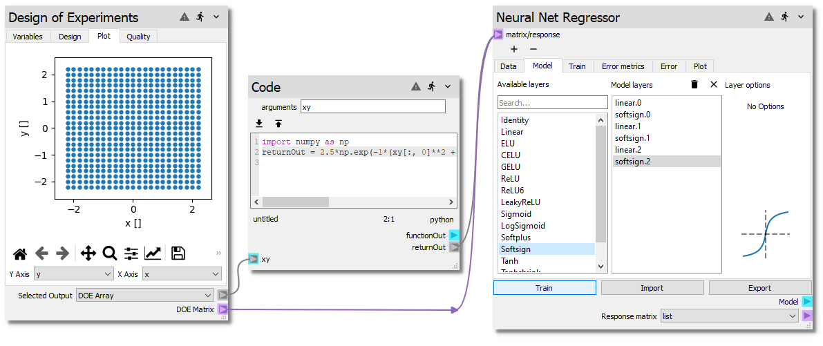
Click over to the Design tab, set the Method to factorial and the
Levels to 23, which will divide the interval between -2.2 and 2.2 into
23 different values of x and y, resulting in 529 total samples. Build the design by clicking on the Build button to
generate the sample. The uniformly spaced factorial design for two input
parameters, which is also referred as a 2D factorial, can be viewed on
the Plot tab, as shown below.
Now we need to evaluate the model at the sampling points. In this case, we are
using the simple function \(r\), which can be easily evaluated with a Code
node following the steps below:
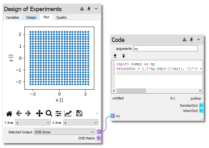
Right click or type to access the node menu and add a Code node.
Set the arguments entry filed at the top of the code node to xy (since
we will pass into the code node an array of the \((x,y)\) values at the
529 design points).
Evaluate the model function \(r\) with python. Non-python users can
simply copy and paste in the code below into the function entry.
Now, we will take the function \(r\) evaluated at the \((x,y)\) sample
points and train a neural network (NN), to approximate the “model” by following these
steps:
Right click or type to access the node menu and add a Neural Network Regressor
node, found in the MachineLearning node collection.
Connect both the DOEMatrix terminal on the Design of Experiments node and
the returnOut terminal of the code node to the matrix/response
terminal of the Neural Network Regressor node.
Next we will build the layers of the NN by going to the Model tab of the
Neural Network Regressor node. Click and drag the layers from the
Availablelayers list to the Modellayers list in the following order:
Linear
softsign
Linear
softsign
Linear
softsign
We will leave the options for the layers at their default settings.
Note
Since the function \(r\) produces both positive and negative values, the
NN needs to end with either an activation function that supports negative
values (like Tanh or Softsign) or a Linear layer. The shape of
the activation function with the default values is displayed under
layeroptions.
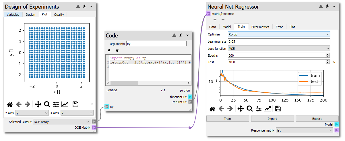
Next, on the Train tab, change the Optimizer to Rprop, the
Lossfunction to MSE and the number of Epochs to 200. Finally,
run the sheet by pressing the button. The samples will be evaluated and
the NN will be trained.
Notice that in the above training plot, once the number of Epochs reaches 100,
the error of the test data no longer reduces. This suggests that any further
training will result in overfitting or memorization of the training data.
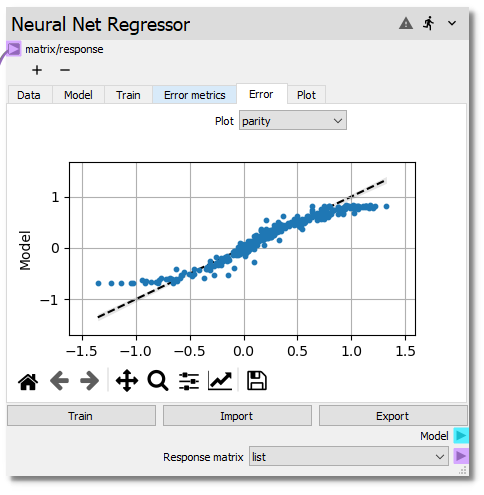
On the Error tab with the Plot type set to “Parity” plot, we can see that the NN has trouble fitting the extremes
(the minimum and maximum of the model). This most likely has to do with the low
sample density at those locations. When Plot type is set to “error”, the
prediction error for each response is plotted. The histogram of errors can be
visualized by setting the Plot type to “histogram”. Ideally for well fitted
model, one would expect to see majority of the errors centered around 0 with low
spread in the histogram.
The plot tab enables both 3D and 2D visualization of the constructed NN model
for qualitative visualization for the two input parameters while superimposing
the actual response values on top of the surface plot.
Now you can play with the layers of the model as well as the training properties
and the model samples. Can you train a better NN to represent the function
\(r\)?
 button to create a new variable. Change the
name to
button to create a new variable. Change the
name to 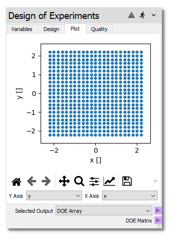
 button. The samples will be evaluated and
the NN will be trained.
button. The samples will be evaluated and
the NN will be trained.