Ex. 1: Surrogate Modeling

Let’s construct a 2D function $r(x,y)$ that’s: linear in $x$, cubic in $y$, exponentially decays away from the origin and has a little noise to mimic realistic responses of a computational model. In the following example we’ll take our “model” to be the simple function defined by:

$$r=2.5(x+y^2+\mathcal{N}(0,0.1))e^{-(x^2+y^2)}$$

In the following steps, we’ll use nodeworks to sample a relevant $(x,y)$ space and construct a surrogate model from responses of the function $r$ evaluated at the sample points.

Sampling

Following the steps below, we’ll create a simple factorial design for sampling the model:

1. Launch Nodeworks and right click on the empty sheet to bring up the menu. Scroll down to Add Node, then down to the Surrogate Modeling and Analysis collection of nodes and (left) click on Design of Experiments to populate the sheet with the Design of Experiments node.

2. On the Variables tab, click the button twice to initiate the $x$ and $y$ variables.

3. By selecting the default entries in thee table, set the variable names to x and y for clarity. (The new entries default to type Double Precision without arg(s) or units and link None, so no change is needed for these properties.)

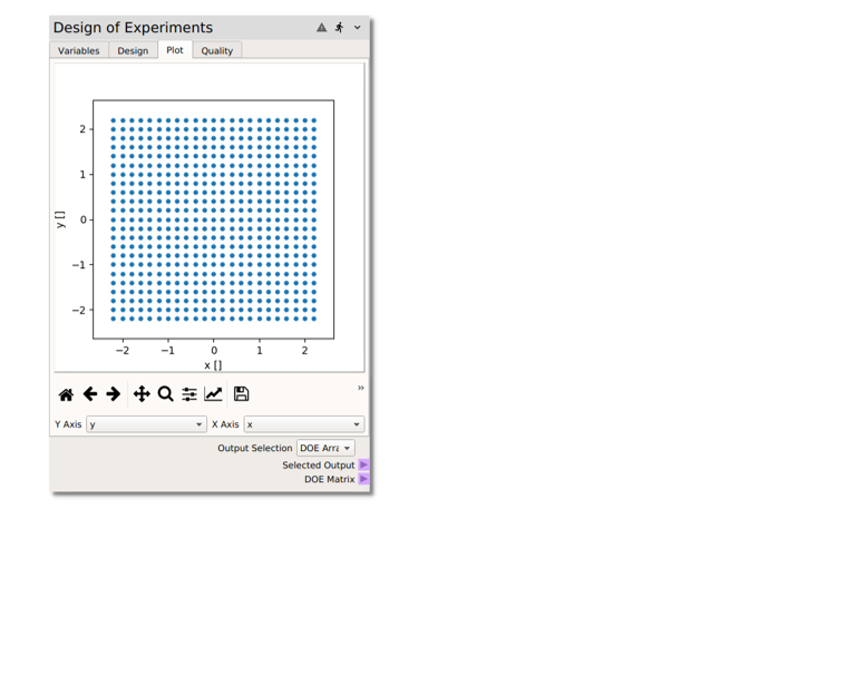
4. We’ll look at a phase space of $(x,y)\in [-2,2]\times [-2,2]$ with a simple interval spacing of 0.2. In order to cover the edges of the domain of interest, set the from and to of both variables to -2.2 and 2.2, respectively. (You can set the levels of each to 23, but we’ll use the same interval for both $x$ and $y$, so variable specific levels won’t be necessary.

5. Click over to the Design tab, set the Method to factorial and the Levels to 23 and click on the Build button to generate the sample. The uniformly spaced 2D factorial design can be viewed on the Plot tab, as shown below.

Model Evaluation

Now we need to evaluate the model at the sampling points. In this case, we are using the simple function $r$, which can be easily evaluated with a code node following the steps below:

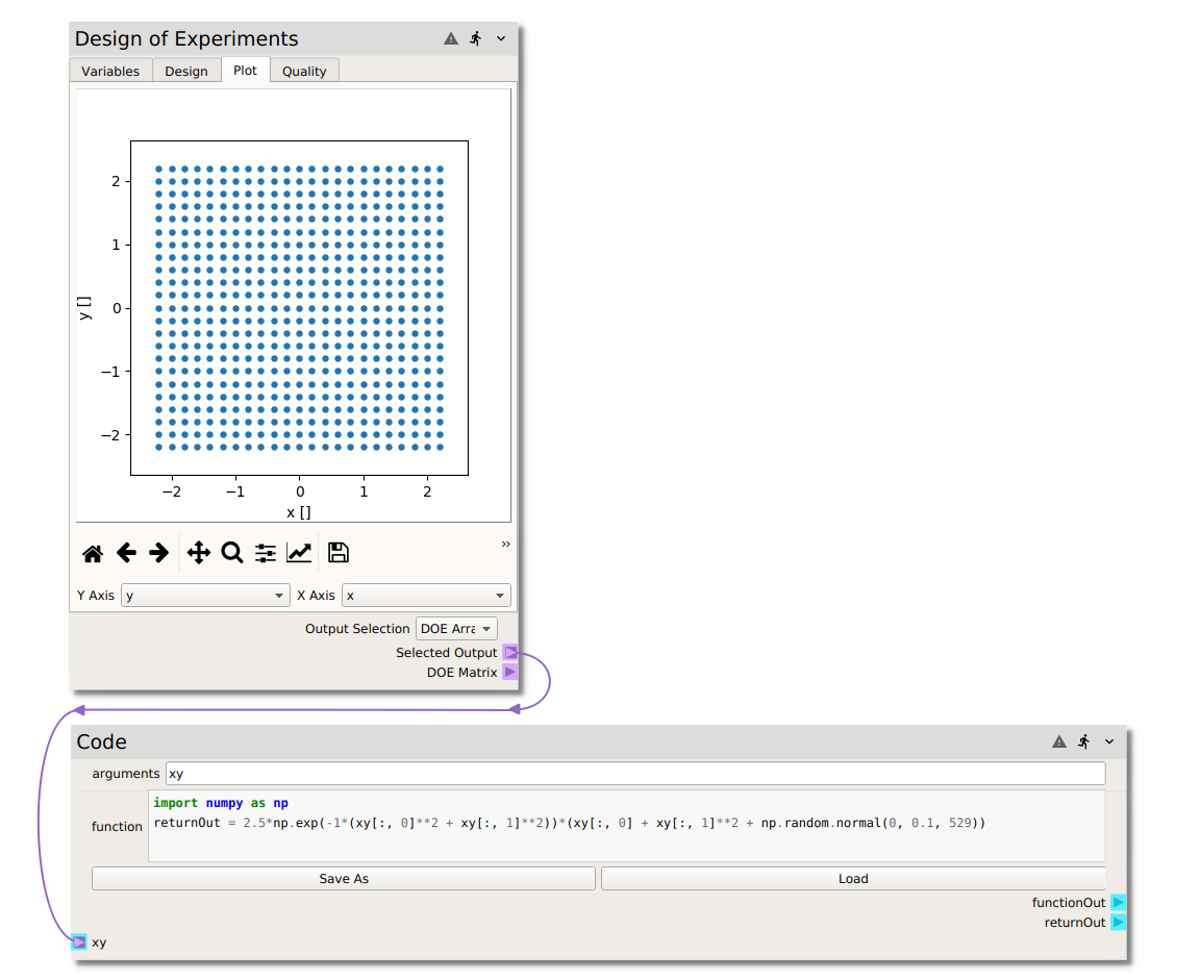
1. Right click or type to access the node menu and add a Code node.

2. Set the arguments to xy (since we will pass into the code node an array of the $(x,y)$ values at the 529 design points).

3. Evaluate the model function $r$ with python. Non-python users can simply copy and paste in the code below into the function entry.

import numpy as np
returnOut = 2.5*np.exp(-1*(xy[:, 0]**2 + xy[:, 1]**2))*(xy[:, 0] + xy[:, 1]**2 + np.random.normal(0, 0.1, 529))

Then

4. Set the Output Selection in the DOE node to DOE Array (our $(x,y)$ array).

5. Add a connection from the Selected Output terminal of the Design of Experiments to the xy terminal of the Code node.

At this point, pressing will send the data from the DOE node to the code node for evaluation. We could connect the code node output to a print node to verify that the function was being evaluated correctly. However in this case (with a previously tested code), we direct the code node output to an RSM node in the section below.

Surrogate Modeling

Now, we will take the function $r$ evaluated at the $(x,y)$ sample points and construct a surrogate model, specifically a Gaussian response surface approximation of the “model” by following these steps:

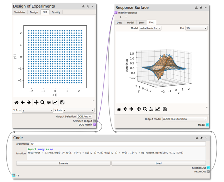
1. Right click or type to access the node menu and add a Response Surface node, found in the Surrogate Modeling and Analysis node collection

2. Connect both the DOE Matrix terminal on the Design of Experiments node and the returnOut terminal of the code node to the matrix/response terminal of the Response Surface node.

3. Click on the Model tab of the Response Surface node and check (under the fit column of the table) the radial basis function model. In the options set the epsilon value to 0.3. For now, the Function and Smooth fields can be left at multiquadric and 0, respectively.

4. Now run the sheet by pressing the button. This will send the data from the DOE node to the code node, calculating the response of the “model” at the sample points, and from there onto the RSM node, constructing a Gaussian process surrogate model. The response data can be viewed in the Data tab in raw table format and in the Plot tab as a 3D surface with response data points from the “actual model” superimposed.

Although we now have a surrogate model, we may want to know:

• How good is this surrogate?

• What is the error in the surrogate relative to the full model?

• Could we build a better surrogate with different model settings a different model option?

We’ll explore these questions in the following section.

(Surrogate) Model Error

The surrogate constructed in the previous section used a multiquadric radial basis function without smoothing, i.e., we left the Smooth parameter at the default 0 value. In this case, the RBF is a pure interpolator. In other words, each sampled point matched exactly by the surrogate. If we click over to the Error tab, you may see a little scatter, but this is only from the (Nodeworks default) 10% holdout for cross validation. If we return to the Model tab and set the cross validation points to 0 and refit the model, the parity plot now shows a perfect 1:1 correlation and the error plot is near single precision numerical zero.

However, it is unlikely that this, essentially error-free, surrogate is the best candidate. Although analysis will not be covered in this example, typically the surrogate will be evaluated at locations in the domain other than the exact sample locations. So, how much error does the surrogate model incur in those instances? One way to answer this is through cross validation. A random sub-set of the data are withheld and the surrogate is fit to the remaining data, the error of which is evaluated with the hold out data. 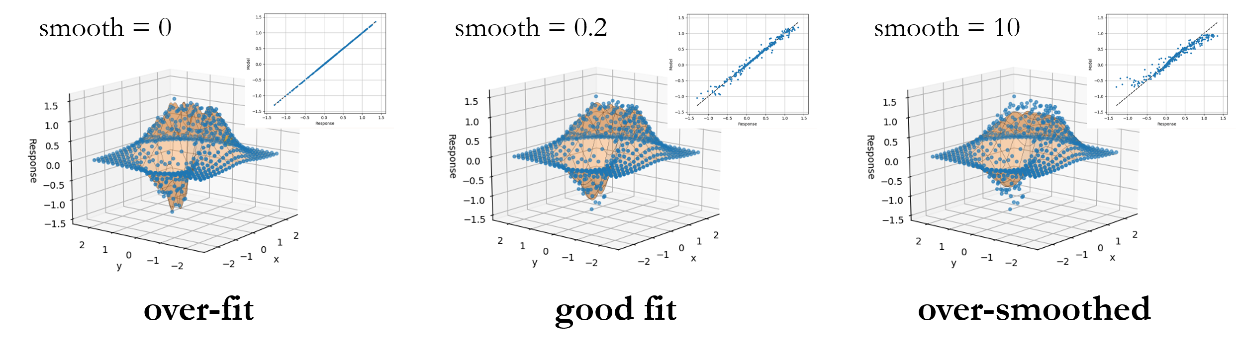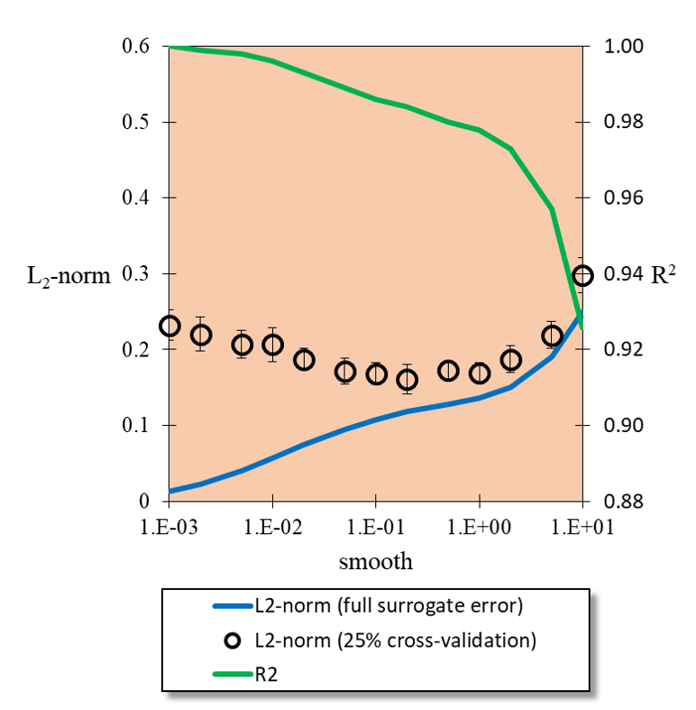To assess the current surrogate model, holdout 25% of the dataset for cross validation and re-fit the model. Repeat this procedure by incrementing the Smooth value and you should notice that the $L_2-norm$ of the error decreases at first before increasing. The image above shows the trends in full surrogate $R^2$ and $L_2$ error, i.e., without cross validation holdout, and the error from 25% cross validation holdout with 95% confidence intervals from 10 replicate cross validation fits. When the RBF acts as an interpolator, i.e., without smoothness, all of the noise from the full model evaluation gets wrapped into the surrogate. (In this case we added our Gaussian noise in intentionally, but in a real simulation this might be due to computational errors such as convergence tolerances, statistical errors, etc.) As the smoothness is increased we stop capturing the noise of each sample until we begin to smooth out some of the underlying function. This is captured in the cross validation as a minimum in the holdout error. Of course wider or tighter stencils, epsilon, or a different radial basis Function or a different surrogate modeling choice altogether may produce an even better fit than the model presented here. Users can test any of the different model options and compare against the surrogate constructed here using the cross validation metrics.