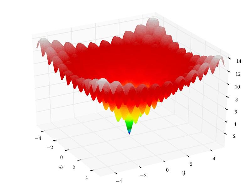
This example demonstrates the optimization of the
Ackley function, which is
commonly used to test the performance of optimization algorithms. The function
has many local minima and one global minimum at \(f(0,0)=0\).
\[f(x,y)=-20exp[{-0.2\sqrt{0.5(x^2+y^2)}}] - exp[{0.5(cos 2 \pi x + cos 2 \pi y)}] + e + 20\]
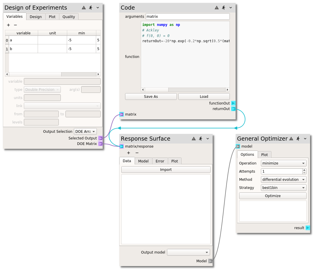
The Node Wizard conveniently provides functionality to populate all the
nodes and provides a collection of optimization test functions, including the
Ackley function. To construct the workflow quickly and focus on the optimization
aspect, use the wizard by:
Click on the button to launch the wizard.
Click on the Optimization tab and set the Functiontobeoptimized
to Ackley and level the Method as surrogate.
Click PopulateNodes
You should now have a collection of nodes including:
a Design of Experiments node with two variables, using the hammersly method with
1000 samples
a Code node with the Ackley function
a Response Surface node with the radialbasisfunction selected, and
Select local from the Method combo-box. The LocalMethod
combo-box should appear with the Nelder-Mead method selected.
Run all the nodes by pressing button on the application toolbar.
After all the nodes have been run, the results of the 10 minimization attempts
are displayed. Notice how each of the 10 attempts seems to provide a different
“optimum”. This happens because each attempt has an initial condition which is
randomly picked from inside the ranges of the variables specified in the
Design of Experiments node. This local minimization method frequently gets stuck in the
many local minima of the Ackley function.
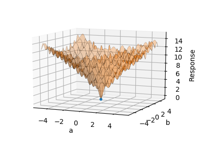
The attempts can be visualized on the Plot tab of the General Optimizer
node, where the surface is the sampled function and the dots are the
optimization attempts. Note how these particular attempts never found the global
minimum:
Global optimization routines try to avoid getting stuck in local minima. One
method provided in the General Optimizer node that works well is
Differential Evolution.
To use this method:
select differentialevolution from the Method combo-box
After the node has run, all 10 optimization attempts should be roughly the same
value, \(f(-0.02, -0.02)=0.19\). The differential evolution algorithm did a
good job of avoiding the local minimas and finding the true minimum.
Unfortunately, this value is not precisely the true minimum, which should be
\(f(0,0)=0\). The problem is that there are not enough samples at or around
the true minimum for the surrogate model, constructed in the Response Surface, to
accurately represent the sharp minimum of the Ackley function.
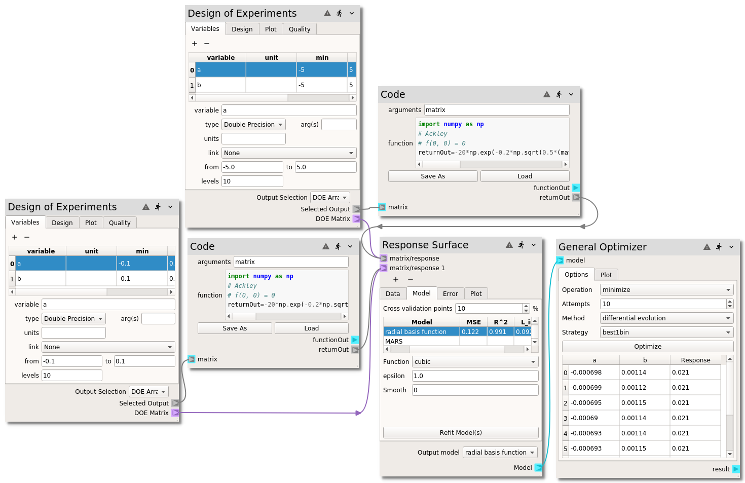
After an optimum has been found, the response surface can be refined around that
optimum to get closer to the true optimum. In this particular case, lets see if
we can get closer to the mathematical optimum. To do this, we will leave the
original samples in-place and add new samples around the optimum:
Select variable a and changed the from value to -0.1 and the
to value to 0.1.
Select variable b and changed the from value to -0.1 and the
to value to 0.1.
On the Design tab, change the number of Samples to 100.
On the Design tab, press the Build button to build the samples.
Adjust the response surface in the Response Surface node node by
Select the Model tab
Select the radialbasisfunction from the table.
Change the Function from multiquadric to cubic
Run all the nodes by pressing button on the application toolbar.
By adding the additional samples, the found optimum
(\(f(-0.0007, 0.001)=0.02\)) is closer to the analytic solution
(\(f(0,0)=0\)). You should have a workflow that looks like this:
Note
See how close you can get to the true solution of \(f(0,0)=0\) by
changing the samples and response surface model settings.
button to launch the wizard.
 button on the application toolbar.
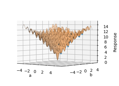
 button below the existing