Ex. 3: Sensitivity Analysis

In this example, we will demonstrate global sensitivity analysis with the aid of a surrogate model. Here, the surrogate will represent a heat exchanger. Sampling of the input parameter space and collection of the response variable (a.k.a. quantity of interest) has already been conducted in a previous study, which we will use to construct a new surrogate model for global SA.

Dataset is generated from the study of Qian et al. [Qian2006] where 64 orthogonal array-based Latin Hypercube design samples where generated for four input parameters, which the study aims to analyze the impact of these factors on heat transfer rates:

No	Variable Name	Symbol	Unit
x1	Mass Flow Rate of entry air	m_flowrate	kg/s
x2	Temp. of entry air	T_in	K
x3	Solid Material Thermal Conductivity	k	W/mK
x4	Temperature of the heat source	T_wall	K

For the details of the study and dataset itself reader is referred to [Qian2006] Table 2 on page 673. The dataset used for this example can be downloaded here in Comma-Separated Values (CSV) format to facilitate import directly to the Response Surface Node. The CSV input file also contains a fifth column, which is the quantity of interest (or response variable), A copy of the input file has been provided at the end of this exercise in tabulated format to facilitate quick review of the imported dataset, which can be also reviewed in detail within the Response Surface Node.

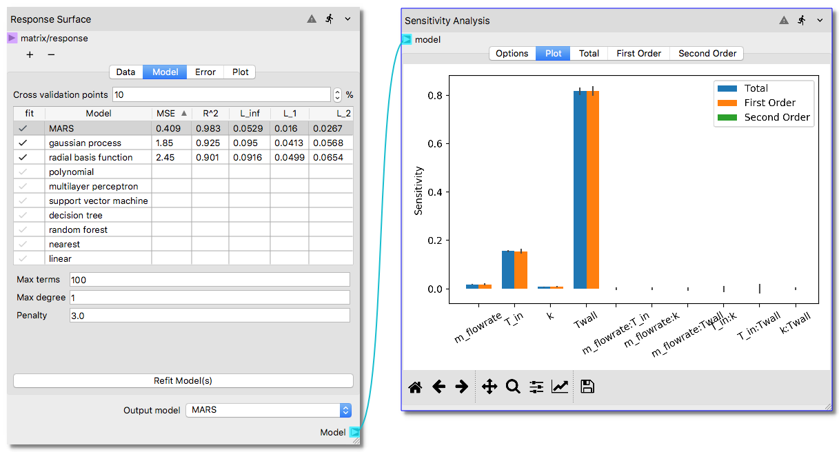
This exercise will show how to construct a surrogate model from an external dataset imported to Nodeworks directly and perform sensitivity analysis to identify the most important input parameters among the four. A completed workflow showing the results of the sensitivity analysis graphically is presented in the following figure.

Build the Surrogate

In this section, we’ll build a surrogate model for the externally created design of experiments. The original DoE employed Latin Hypercube sampling based design for space filling property. The corresponding response variables were computed with finite difference simulations. The SA aims to determine which of the input parameters among the four has the most influence in the response variable.

1. Right click somewhere in the blank worksheet then click Add Node and then Surrogate Modeling Analysis option to select and add a Response Surface node as shown in the figure below.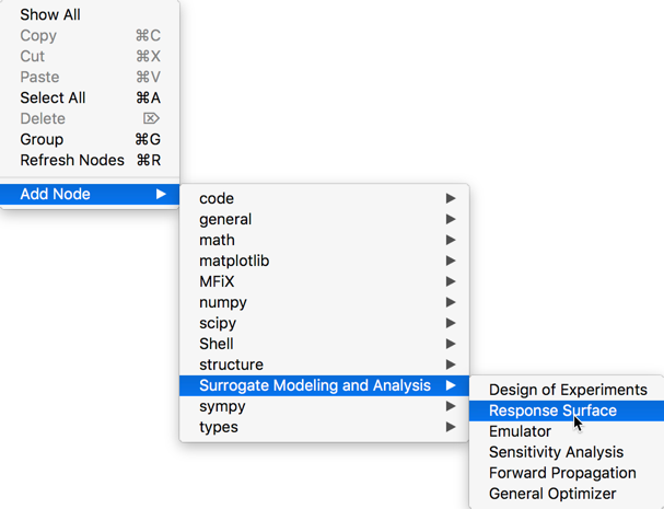

   

2. In the Response Surface node click on the Import button in the first tab under Data This will open a new window titled Read CSV File as shown below.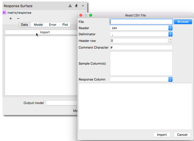

   

3. Select the datafile in CSV format, which contains the 64 sample Latin Hypercube for four parameters (m_flowrate, T_in, k, and T_wall) and one response variable (y_a) by clicking the Browse button. Once the correct file is located, the available dataset will be previewed in the window. Unclick the last entry y_a to remove from the Sample Columns list which is used to designate which columns in the file will be treated as input parameters. In the entry for Response Column, use the scroll bar on the right side to scroll down and select y_a as the response variable. To import the dataset into Nodeworks click Import button after making the above changes in the window.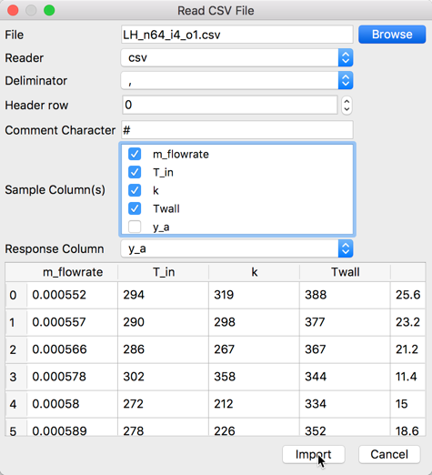

   

   After successfully importing the dataset, the Response Surface node should show the imported dataset under Data tab as shown for the first 20 rows in following figure.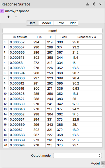

   

4. Next step involves testing different surrogate model methods to assess the best data-fitted surrogate for the given dataset. In the Response Surface node, click on the Model tab and set the Cross validation points to 0. Next check and highlight several surrogate model options that is expected to give best fit. For this example, we will select gaussian process, polynomial, linear, radial basis function, and MARS. Note that the wall clock time required to construct surrogate models with more options may noticeably increase as the sample size substantially increases (e.g., from 64 to 10000 samples). Each surrogate model option comes with its own set of parameters for tuning the process, which will not be changed for this example, and the defaults will be accepted. However, user is encouraged to understand these parameters and explore their effect while in pursuit of the best data-fitted surrogate model at this phase. The selection of the surrogate models before initiating the process for construction are shown below.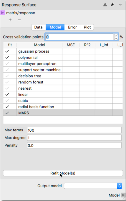

To initiate the surrogate model construction process hit Refit Model(s) button where the mouse cursor in the above figure is placed. After the process is completed user should see surrogate model quality metric calculated as shown below. Note that you may need to enlarge the node towards right side to be able to see the additional metrics shown in the figure. Clicking the header of any column triggers sort based on the numeric values in that column, which helps to better assess which method achieved the best fit based on the surrogate model quality metric such R ².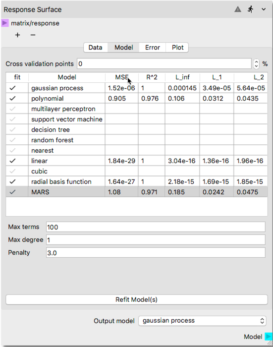

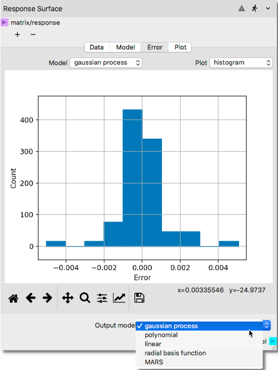
After reviewing the metrics to assess the quality of the fitted response and/or graphical visualizations showing the error for fitted response surface predictions at the actual sample locations, select the best suitable response surface in the Output Model field at the right bottom using the scroll bar as shown in the below illustration.

5. After constructing an adequate response surface to characterize the relationship between input and outputs, add a Sensitivity Analysis node from Surrogate Modeling and Analysis collection of the node library.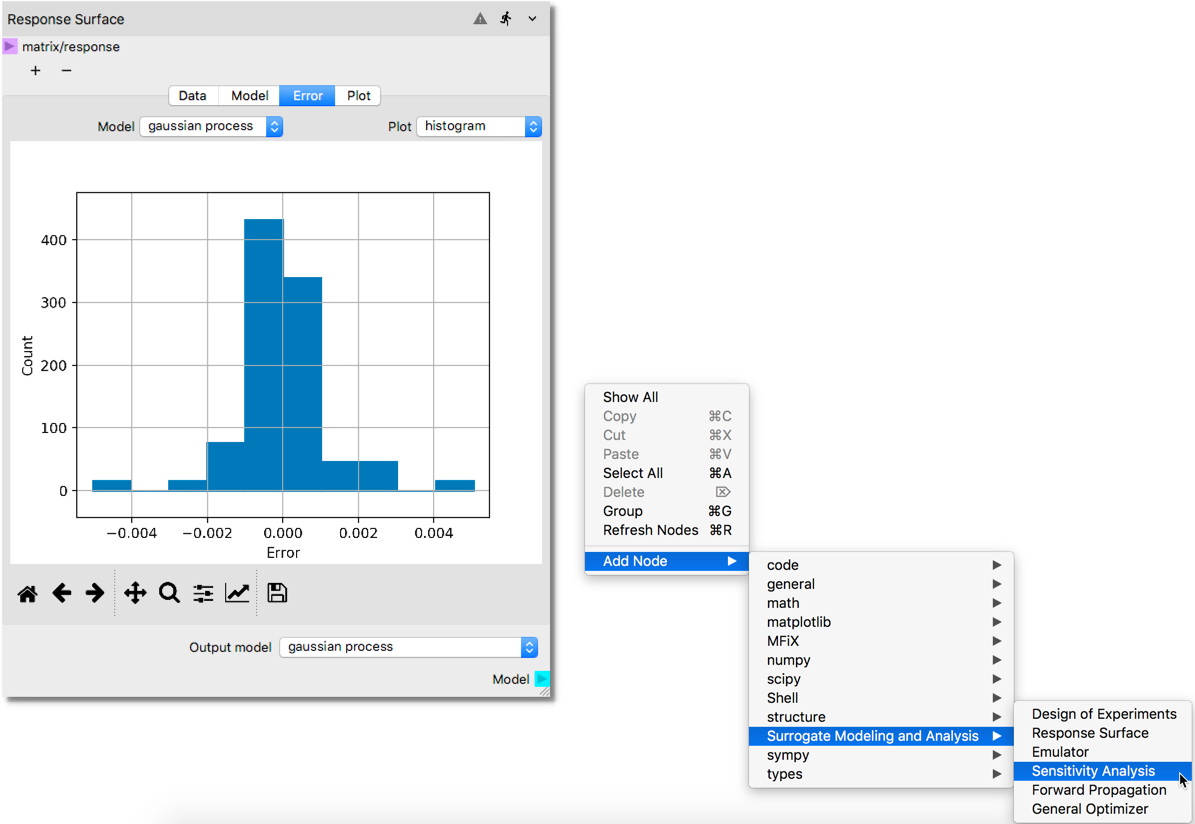

Then, connect the Model terminal of the Response Surface node to the model terminal of the Sensitivity node, as shown in the illustration below.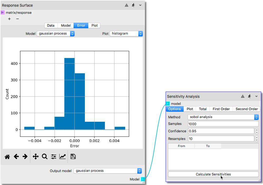

To start the Sensitivity Analysis, click Calculate Sensitivities at the bottom of the Options tab. As shown below, it will retrieve the input parameter dataset from the Response Surface Node. The lower and upper bounds of the input parameters will be displayed in this tab after the completion of analysis.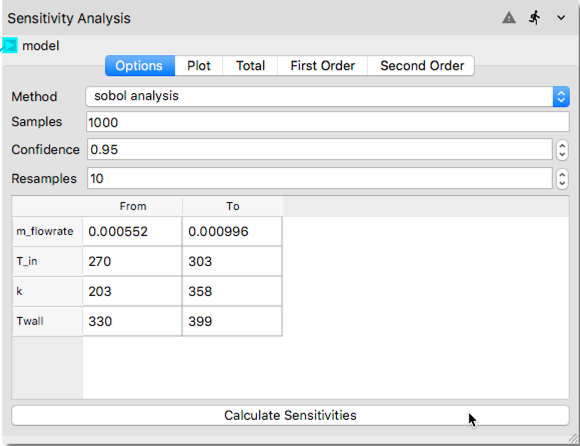

The results of the Sensitivity Analysis can be visualized in the Plot tab. As shown in the following illustration, after clicking the Plot tab a bar chart is created. First order Sobols’ indices show the main effects, i.e., the effect of the each input parameter considered standalone. The second order indices show the interaction effects such as interaction of mass flow rate with inlet temperature (labeled as m_flowrate:T_in in the x-axis of the bar chart). Total indices shown with blue color is an aggregate result for the overall effect of each input parameter. The bar chart shows that among the four input parameters, the wall temperature has the most influence on the system response.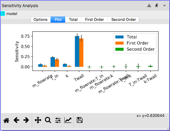

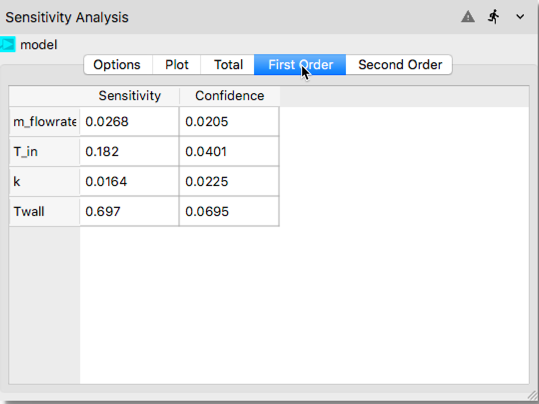
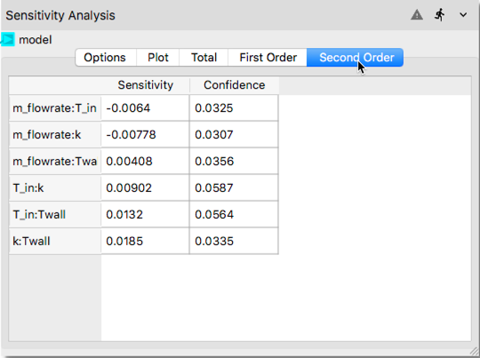
The remaining tabs in the Sensitivity Analysis node (i.e., Total, First Order and Second Order) show quantitatively the values of the sensitivity indices displayed graphically in Plot tab in a tabulated format as shown in the following figures.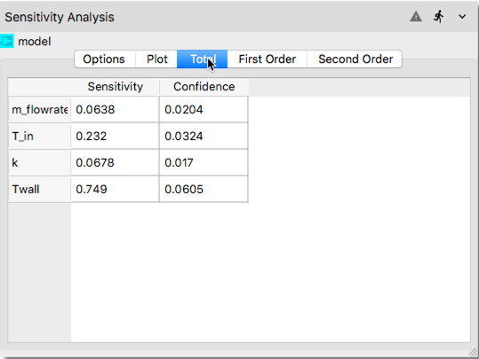

In the tabulated data compiled, first and second columns show the computed Sobols’ indices and confidence interval, respectively.

References:

[Qian2006] (1,2)

Qian, Zhiguang, Carolyn Conner Seepersad, V. Roshan Joseph, Janet K. Allen, and CF Jeff Wu. “Building surrogate models based on detailed and approximate simulations.” Journal of Mechanical Design 128, no. 4 (2006): 668-677.

External Dataset:

The contents of data/LH_n64_i4_o1.csv

x1	x2	x3	x4	y1
m_flowrate	T_in	k	Twall	y_a
0.000552	293.53	318.63	388.29	25.61
0.000557	290.18	298.27	377.49	23.24
0.000566	285.77	266.71	367.27	21.23
0.000578	302.17	358.13	343.72	11.44
0.00058	272.26	211.71	333.65	15.03
0.000589	278.16	225.78	351.83	18.55
0.000594	279.54	258.51	360.13	20.74
0.000603	296.75	323.15	399.45	28.4
0.000612	280.83	291.53	394.72	30.22
0.000615	300.28	270.74	335.79	9.53
0.000626	284.89	350.46	352.29	18.13
0.000627	287.6	243.96	382.54	25.02
0.000639	270.45	241.21	341.81	17.92
0.000643	276.17	216.99	371.6	24.2
0.000652	298.04	303.96	361.58	17.47
0.000657	294.24	330.63	375.53	22.48
0.000669	296.33	343.16	385.81	25.07
0.00067	303.07	321.41	370.48	18.93
0.000683	287.05	227.31	358.24	18.61
0.000689	272.7	260.91	355.37	21.31
0.000694	278.35	212.79	376.24	25.11
0.000698	277.52	299.39	338.4	16.02
0.000711	292.26	273.31	392.54	27.47
0.000714	283.08	306.69	344.34	16.43
0.000722	276.53	353.75	374.41	26.5
0.00073	285.51	217.74	383.92	25.88
0.000738	295.01	295.02	347.22	14.37
0.000741	270.95	275.19	356.87	22.36
0.000751	287.99	326.02	354.08	18.17
0.000757	300.64	235.03	391.68	14.37
0.000763	292.82	254.84	373.38	21.96
0.000772	278.93	301.75	331.55	14.02
0.000782	299.86	317.84	348.41	13.68
0.000786	275.51	247.29	340.19	16.82
0.000791	271.64	284.88	365.09	25.06
0.0008	291.42	341.48	358.59	18.83
0.000803	281.47	232.64	389.46	28.69
0.000814	286.39	339.92	332.4	12.68
0.000823	288.53	207.55	393.49	27.96
0.000828	297.33	280.13	379.86	23.17
0.000836	289.62	347.65	335.44	12.79
0.000842	294.39	203.45	346.05	13.75
0.000851	273.71	315.27	381.14	29.08
0.000857	282.12	262.3	350.1	18.25
0.000865	274.35	335.16	362.3	23.89
0.00087	295.76	237.65	366.25	19.36
0.000874	282.5	253.25	396.36	30.9
0.000882	299.22	288.45	385.07	24.45
0.000891	273.43	336.04	386.95	31.05
0.000901	302.02	249.57	382.33	22.64
0.000903	284.25	290.9	364.99	22.22
0.000911	280.17	355.34	370.03	25.03
0.00092	276.89	310.73	397.78	33.27
0.000929	298.65	205.4	349.02	13.67
0.000934	288.86	265.53	339.54	13.89
0.000943	292.77	231.01	330.19	10.16
0.000947	283.62	222.95	378.66	25.48
0.000956	290.33	312.97	368.96	22.22
0.000964	271.23	348	398.52	35.05
0.000968	297.8	244.5	337.41	10.99
0.000979	291.21	283.1	353.6	17.45
0.000985	301.5	220.37	363.2	17.14
0.000987	281.11	329.45	342.32	16.95
0.000996	275.01	278.27	390.35	31.35