8.4. Frequently Asked Questions¶
This document explains how to perform common tasks with MFiX.
8.4.1. How do I ask question, or send feedback?¶
Please send specific questions and feedback regarding the GUI to the support forum. Please include your version info in all communications (Menu –> About and press the “Copy Version Info” button). Other technical questions regarding MFiX can be sent to the support forum.
8.4.2. How do I change the look & feel of the GUI?¶
Go to the Settings pane and change the style from the pull down menu.
8.4.3. MFiX (VTK) crashes on RHEL/CentOS 7 with the following error message:¶
ERROR: In ../Rendering/OpenGL2/vtkShaderProgram.cxx, line 431
vtkShaderProgram (0x55555dda47a0):
This error message means that the OpenGL driver in RHEL 7.5 does not support the version needed by VTK.
Try using an earlier version of OpenGL:
env MESA_GL_VERSION_OVERRIDE=3.2 mfix
If this solves the issue for your system, you can add export
MESA_GL_VERSION_OVERRIDE=3.2 to your shell profile.
8.4.4. How do I build the custom solver in parallel?¶
The custom solver can be built in parallel from the GUI by checking the “Build solver in
parallel” check box. This will pass the -j option to the make command and
significantly decrease the time to build the solver.
8.4.5. Play/Pause/Reinit¶
While the simulation is running, it can be paused by pressing the  (pause) button.
Many settings can be modified, such as stop time, monitor and VTK settings, boundary conditions, etc.
Settings that cannot be changed (such as initial conditions or grid spacing) will be disabled while the simulation is paused.
To resume the simulation, save the new settings by pressing the
(pause) button.
Many settings can be modified, such as stop time, monitor and VTK settings, boundary conditions, etc.
Settings that cannot be changed (such as initial conditions or grid spacing) will be disabled while the simulation is paused.
To resume the simulation, save the new settings by pressing the  (save) button
and press the
(save) button
and press the  (start) button.
8.4.6. Restart a simulation from current time¶
Once a simulation has run to completion, it can be restarted from the current simulation time.
Increase the stop time in the “Run” pane, press the (save) button,
and press the (start) button. In the “Run solver” dialog box, check the “Restart”
check box and select “Resume”. Then press the “Run” button.
8.4.7. Restart a simulation from the beginning¶
Once a simulation has run to completion, or if you pressed the  (stop) button,
the simulation can be restarted from the beginning. This is typically needed if the simulation
settings need to be changed and the current results are not needed anymore.
First press the
(stop) button,
the simulation can be restarted from the beginning. This is typically needed if the simulation
settings need to be changed and the current results are not needed anymore.
First press the  (reset) button to delete the current results. Next change the simulation
settings as needed (if any). Press the (save) button, and press the (start) button.
(reset) button to delete the current results. Next change the simulation
settings as needed (if any). Press the (save) button, and press the (start) button.
8.4.8. What system of units does MFiX use?¶
Simulations can be setup using the International System of Units (SI). The centimeter-gram-second system (CGS) is no longer supported.
Property |
MFiX SI unit |
|---|---|
length, position |
meter \((m)\) |
mass |
kilogram \((kg)\) |
time |
second \((s)\) |
thermal temperature |
Kelvin \((K)\) |
energy† |
Joule \((J)\) |
amount of substance‡ |
kilomole \((kmol)\) |
force |
Newton (\(N = kg·m·s^{-2}\)) |
pressure |
Pascal (\(Pa = N·m^{-2}\)) |
dynamic viscosity |
\(Pa·s\) |
kinematic viscosity |
\(m^2·s^{-1}\) |
gas constant |
\(J·K^{-1}·kmol^{-1}\) |
enthalpy |
\(J\) |
specific heat |
\(J·kg^{-1}·K^{-1}\) |
thermal conductivity |
\(J·m^{-1}·K^{-1}·s\) |
† The SI unit for energy is the Joule. This is reflected in MFiX through the gas constant. However, entries in the Burcat database are always specified in terms of calories regardless of the simulation units. MFiX converts the entries to joules after reading the database when SI units are used.
‡ The SI unit for the amount of a substance is the mole (mol). MFiX uses the kilomole (kmole). These units are needed when specifying reaction rates:
amount per time per volume for Eulerian model reactions (kmole.s^{-1}.m^3)
amount per time for Lagrangian model reactions (kmole.s^{-1})
8.4.9. What do I do if a run does not converge?¶
Initial non-convergence:
Ensure that the initial conditions are physically realistic. If in the initial time step, the run displays NaN (Not-a-Number) for any residual, reduce the initial time step. If time step reductions do not help, recheck the problem setup.
Holding the time step constant (DT_FAC=1) and ignoring the stalling of
iterations (DETECT_STALL=.FALSE.) may help in overcoming initial nonconvergence.
Often a better initial condition will aid convergence. For example, using a
hydrostatic rather than a uniform pressure distribution as the initial condition
will aid convergence in fluidized bed simulations.
Often a better convergence is achieved with ideal gas law than with constant gas density. If poor convergence or failure to converge is observed while using constant gas density, it is recommended to switch to ideal gas law. In this case the average molecular weight or individual gas species molecular weights must be defined, and gas pressure and temperature must be defined in all initial and boundary condition regions.
If there are computational regions where the solids tend to compact (i.e.,
solids volume fraction less than EP_star), convergence may be improved by
reducing UR_FAC(2) below the default value of 0.5.
Convergence is often difficult with higher order discretization methods. First order upwinding may be used to overcome initial transients and then the higher order method may be turned on. Also, higher-order methods such as van Leer and minmod give faster convergence than methods such as superbee and ULTRA-QUICK.
Non-convergence due to bad cut-cell mesh:
When using cut-cells, non-convergence can arise due to a few bad cut cells, typically small cells (in volume) or bad cut cells coming from poorly resolved geometry in a coarse mesh with geometrical details in the order of one to two cells.
Convergence may be improved by lowering the number of small cut cells. This can be done either by removing small cut cells or by snapping intersection points to cell corners. The settings are available in the Mesh> Mesher pane in the GUI, or through keywords in the .mfx file.
To completely remove a small cut cell, increase the “small cell tolerance” (default value is 0.01), or modify the TOL_SMALL_CELL keyword when editing the .mfx file.
To snap intersection points to a cell corner, increase the “snap tolerance” (default value is 0.00), or modify the TOL_SNAP keyword when editing the .mfx file.
Increasing the “small area tolerance” (TOL_SMALL_AREA keyword) or Normal distance tolerance (TOL_DELH keyword) may also help.
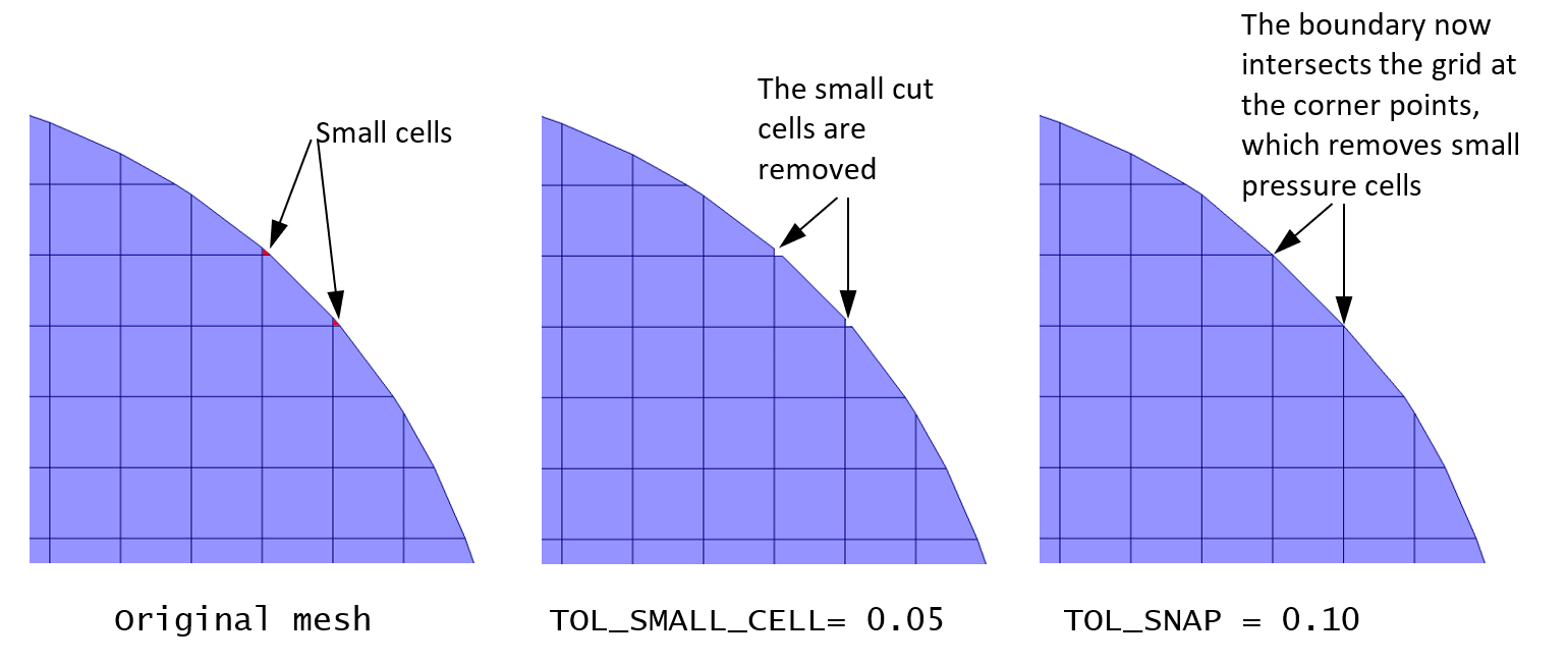
Fig. 8.3 Removing small cut-cells¶
8.4.10. How to provide initial particle positions in particle_input.dat file?¶
We can read the initial particle data from a text file, called particle_input.dat.
The format of this file has changed in the 20.3 release. The old file version can still
be used but it is recommended to use the latest format.
To use the file rather than the automatic particle generation (i.e. from Initial Conditions regions), go to the Solids > DEM pane, and leave the “Enable automatic particle generation” checkbox unchecked. Enter a positive number of particles to be read in the “Data file particle count”.
Version 2.0 (MFiX 20.3 release)
The new format allows to either read variables or set a constant value for all particles. The file contains a long header where information about the data is specified. This controls how many columns and which variables are read from the file. Next, the data section contains the data for each particle. Each column corresponds to a variable. In 3D, the first 3 columns are always the x,y and z coordinates of the particle’s center. In 2D, the first 2 columns are always the x,y coordinates of the particle’s center. There are two options for the other variables: either read the data for each particle in the next column, or assign a constant value to all particles.
Below is an example of a particle_input.dat file (the line number is shown on the left and it
not part of the data itself):
Line 1 : File version. Do not change this line.
Lines 2-18 : Instructions to use the file.
Line 19 : This is a 3D geometry. The first 3 columns in the data section will be x,y,z.
Line 20 : We will read data for 35361 particles.
Line 24 : We always read coordinates in the first 2 or 3 columns (do not change)
Line 25 : We do not read particle’s phase ID for each particle. It is assigned a constant value: 1
Line 26 : We will read the particle’s diameter in the next column (column#4).
Line 27 : We do not read particle’s density. It is assigned a constant value: 2500.0 kg/m^3
Line 25 : We do not read particle’s velocity. It is assigned a constant value: (u,v,w) = (0.0,0.0,0.0) m/s
Lines 29-30: This is a cold, non reacting case, we do not read Temperature or species.
Line 31 : We do not have user scalars, so we do not read them.
Lines 32-34: Data header
The data starts on Line 35. Based on the above settings, we need to read, x,y,z, and the diameter of each particles, i.e., 4 columns, for 35361 particles. Only the first few lines of the data is shown.
1 Version 2.0
2 ========================================================================
3 Instructions:
4 Dimension: Enter "2" for 2D, "3" for 3D (Integer)
5 Particles: Number of particles to read from this file (Integer)
6 For each variable, enter whether it will be read from the file
7 ("T" to be read (True), "F" to not be read (False)). When not read, enter the
8 default values assign to all particles.
9 Coordinates are always read (X,Y in 2D, X,Y,Z in 3D)
10 Phase_ID, Diameter, Density, Temperature are scalars
11 Velocity requires U,V in 2D, U,V,W in 3D
12 Temperature is only read/set if the energy equation is solved
13 Species are only read/set if the species equations are solved, and requires
14 all species to be set (if phase 1 has 2 species and phase 2 has 4 species,
15 all particles must have 4 entries, even phase 1 particles (pad list with zeros)
16 User scalars need DES_USR_VAR_SIZE values
17 Data starts at line 35. Each column correspond to a variable.
18 ========================================================================
19 Dimension:    3
20 Particles:    35361
21 ========================================================================
22 Variable      Read(T/F)     Default value (when Read=F)
23 ========================================================================
24 Coordinates:     T          Must always be T
25 Phase_ID:        F          1
26 Diameter:        T
27 Density:         F          2500.0
28 Velocity:        F          0.0 0.0 0.0
29 Temperature:     T          (Ignored if energy eq. is not solved)
30 Species:         T          (Ignored if species eq. are not solved)
31 User_Scalar:     T          (Ignored if no user scalars are defined)
32 ========================================================================
33     X (m)           Y (m)           Z (m)       Diameter (m)
34 ========================================================================
35 -5.07749E-02    -7.98147E-01    -2.00612E-01    9.71052E-03
36 -4.86164E-02    -8.16202E-01    -2.25035E-01    8.34185E-03
37 -3.16460E-02    -8.13702E-01    -2.19164E-01    1.09747E-02
38 -3.32833E-02    -8.25178E-01    -2.19393E-01    9.67983E-03
39 -2.48844E-02    -8.30159E-01    -2.16423E-01    9.84182E-03
40 -8.57591E-03    -8.38121E-01    -2.08773E-01    9.92759E-03
41 -2.75312E-03    -8.32665E-01    -2.00770E-01    1.07560E-02
42 1.57276E-02     -8.37839E-01    -2.08196E-01    1.04387E-02
43 1.96605E-02     -8.31447E-01    -2.15105E-01    9.97808E-03
44 2.71083E-02     -8.26450E-01    -2.19492E-01    9.99619E-03
45 3.55440E-02     -8.28885E-01    -2.15687E-01    9.15771E-03
46 4.45244E-02     -8.28239E-01    -2.11771E-01    1.05089E-02
47 4.70488E-02     -8.22092E-01    -2.19129E-01    9.33350E-03
The particle_input.dat file can be edited in any text editor, including the GUI editor, and be
saved in the project directory. Please run the 2D DEM fluid bed with central jet tutorial from the GUI, or see the DEM Initial Conditions last section for an example.
Version 1.0 (Prior to MFiX 20.3 release)
The file stores each particle position, radius, density, and velocity. For 2D geometries, it contains 6 columns: x , y, radius, density, u, v. In 3D, it contains 8 columns: x , y, z, radius, density, u, v, w. The number of lines correspond to the number of particles read, and should match the “Data file particle count” defined in the Solids > DEM tab. The check box “Enable automatic particle generation” must be left unchecked.
Below is an example of a 2D particle_input.dat (only 4 particles shown):
0.2000D-03  0.2000D-03  0.5000D-04  0.1800D+04  0.0000D+00  0.0000D+00
0.6000D-03  0.2000D-03  0.5000D-04  0.1800D+04  0.0000D+00  0.0000D+00
0.1000D-02  0.2000D-03  0.5000D-04  0.1800D+04  0.0000D+00  0.0000D+00
0.1400D-02  0.2000D-03  0.5000D-04  0.1800D+04  0.0000D+00  0.0000D+00
Below is an example of a 3D particle_input.dat (only 4 particles shown):
0.2000D-03  0.2000D-03  0.1000D-01  0.5000D-04  0.1800D+04  0.0000D+00  0.0000D+00  0.0000D+00
0.6000D-03  0.2000D-03  0.1000D-01  0.5000D-04  0.1800D+04  0.0000D+00  0.0000D+00  0.0000D+00
0.1000D-02  0.2000D-03  0.1000D-01  0.5000D-04  0.1800D+04  0.0000D+00  0.0000D+00  0.0000D+00
0.1400D-02  0.2000D-03  0.1000D-01  0.5000D-04  0.1800D+04  0.0000D+00  0.0000D+00  0.0000D+00
8.4.11. How to verify/flip STL file facet normals?¶
When using an STL file to define the geometry, a normal vector is associated with each facet (triangle). The direction in which the normal vector points indicates the fluid region. It is important to verify the normal vectors points in the desired direction before running the simulation.
To show the normal vectors in the Model view, expand the geometry view settings on the right and check “Show Normals”. It may be necessary to adjust the scale to get a better view. The figure below shows an example of a cylinder with vectors pointing towards the interior region of the cylinder. This will correspond with an internal flow simulation where the fluid region is located inside the cylinder and the outside region is not part of the simulation.
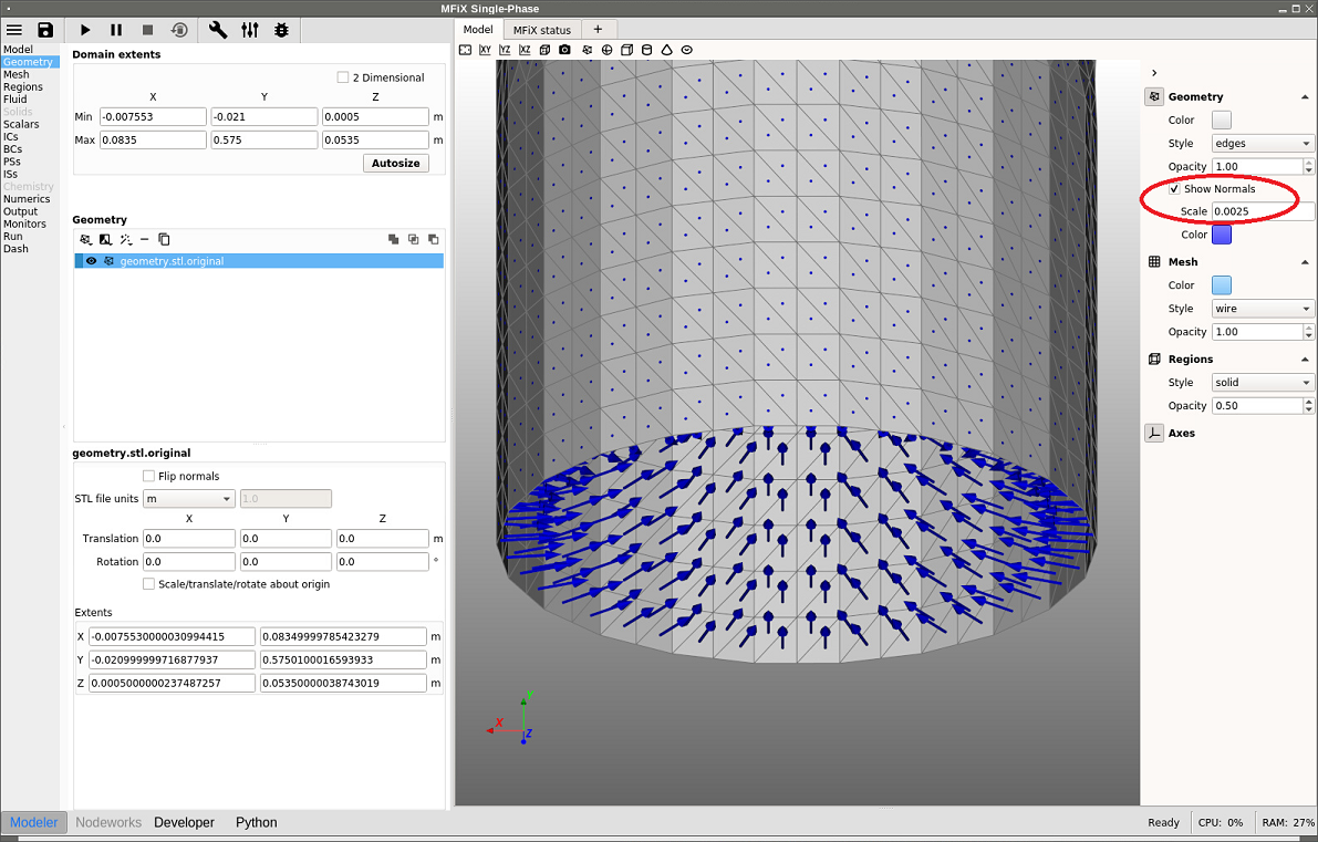
Fig. 8.4 Displaying STL normals, internal flow¶
If the normal vectors are not pointing in the correct direction, the normals can be flipped by checking the “Flip normal” box for any selected stl file. To model an external flow using the same geometry as above, flip the normals and the change will be reflected in the Model view (see figure below). Now the normals points towards the outside of the cylinder, and the region inside the cylinder will not be part of the computation.
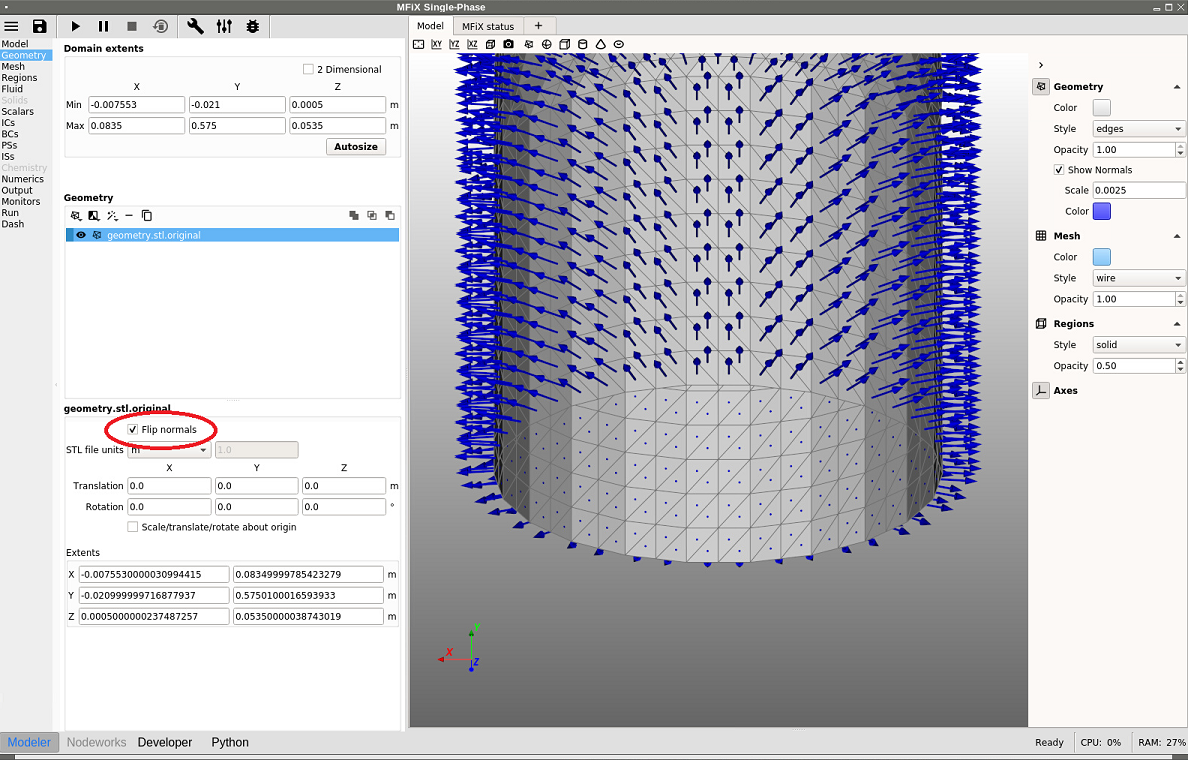
Fig. 8.5 Flipping STL normals to model an external flow¶
8.4.12. How to manually specify a grid partition for DMP runs?¶
When running a simulation in parallel (DMP) mode, the parallel decomposition is by default uniform in each direction and the number of partitions is set by NODESI, NODESJ, and NODESK in the x,y and z directions, respectively. The default partition may not always be the most efficient. For example, a DEM simulation of a fluidized bed where most particles are at the bottom of the bed may run faster if smaller partitions are set at the bottom, where many particles are located and a large partition is used in the freeboard. This will better distribute particles among processors, and provide a better load balance.
Let’s assume the mesh contains 20x100x20 cells (IMAX=20, JMAX=100, KMAX=20) and we use 16 cores with a 2x4x2 partition (NODESI=2, NODESJ=4, NODESK=2). Assume particles are roughly located within the bottom half of the bed throughout the simulation. With the default (uniform) decomposition, each vertical partition will contain JMAX/NODESJ=25 cells (Figure 8.6). This means 8 cores will remain mostly idle with respect to particle tracking and collision.
Instead, we can distribute cells in the y-direction so that the vertical partitions have roughly the same number of particles. This can be achieved with 10, 10, 10, and 70 cells from bottom to top. (Figure 8.7).
Due to the symmetry of the problem in x and z directions, no adjustment is needed in these directions, and a uniform distribution is adequate.
Note that the custom partition will provide better load balance for particles but will make the fluid calculation slower since fluid cells will be unbalanced. However, since a large majority of the time is spent in the DEM loop, it should be beneficial to customize the partition.
To specify this decomposition, the following gridmap.dat needs to be saved in the project directory:
The first line specifies the values of NODESI, NODESJ, NODESK.
2 4 2 ! NODESI, NODESJ, NODESK
The next two lines (NODESI=2) specify the partition sizes in the x-direction. Here each partition contains 10 cells:
0        10
1        10
The next four lines (NODESJ=4) specify the partition sizes in the y-direction. Here three partitions at the bottom contains 10 cells each, and the last partition contains 70 cells:
0        10
1        10
2        10
3        70
The last two lines (NODESK=2) specify the partition sizes in the z-direction. Here each partition contains 10 cells:
0        10
1        10
Below is the entire gridmap.dat file:
2        4          2    ! NODESI, NODESJ, NODESK
0        10
1        10
0        10
1        10
2        10
3        70
0        10
1        10
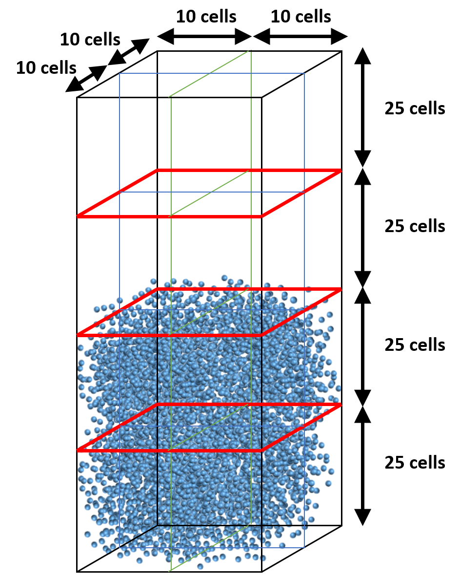
Fig. 8.6 Default partition (uniform distribution)¶
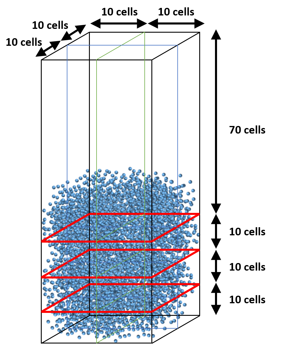
Fig. 8.7 Adjusted partition in vertical direction (specified with gridmap.dat)¶
8.4.13. How to avoid particles going through solid walls in DEM simulations?¶
This is a common issue that arises when particles are too soft. Increasing the spring stiffness (kn and kn_w) typically helps resolve the issue.
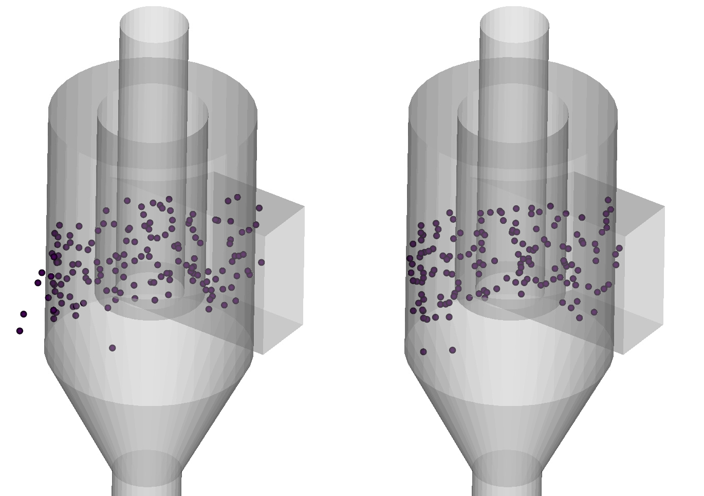
Fig. 8.8 Left: Soft particles (kn=kn_w=100 N/m) going through the cyclone wall. Right: Harder particles (kn=kn_w=1000 N/m) bouncing off the wall.¶
The spring stiffness can be adjusted in the Solids>DEM pane:
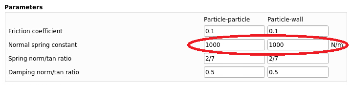
Fig. 8.9 Spring stiffness settings in the GUI¶
Other possible reasons DEM particles may go through the wall:
Missing facets from the STL files: If the STL file is not waterproof, particles can go through the holes. The STL file must be inspected and corrected to fix this issue. The STL file should also not have facets with an angle smaller than the facet angle tolerance (Mesh> mesher pane).
DEM solids time step is too large. If the DEM solids time step is too large, collisions may be missed and particles can go through the wall. Increasing the spring stiffness will automatically reduce the solids time step, but it may be necessary to increase the DEM time step factor (Solids>DEM pane). It is recommended to not lower the DEM time step factor below the default value of 50.