MFiX Examples

Ex. 1: Single Phase Solution Verification

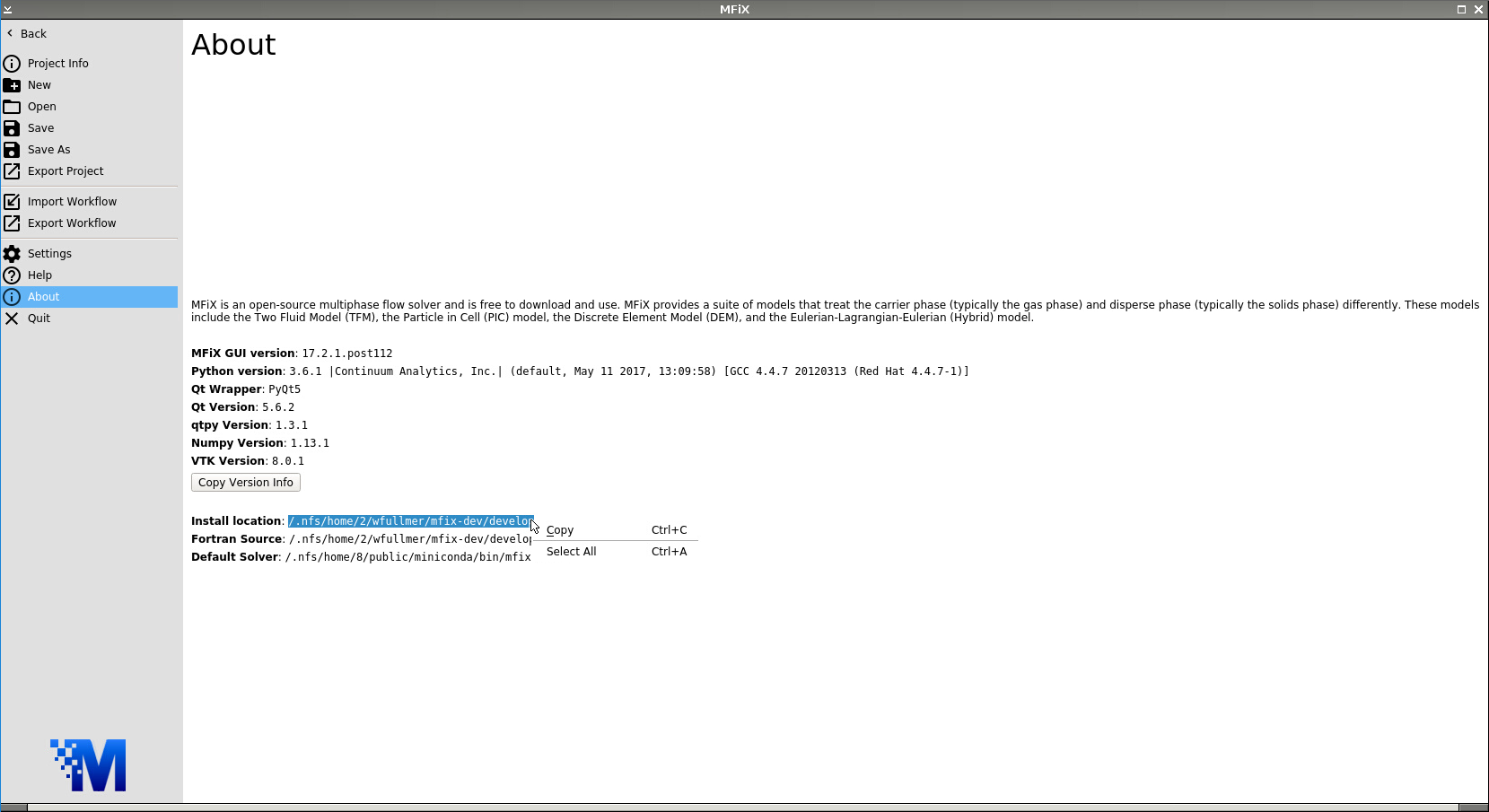
In this first test of the MFiX-Nodeworks interface, we’ll run a simple solution verification test problem of plane Poiseuille flow. An input file for this case has already been distributed with MFiX which we will use. First, launch a new instance of MFiX. Navigate to the About tab of the main File Menu to find the Install location. Highlight and copy this path.

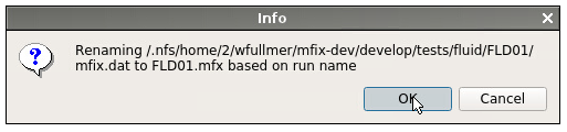
Now, navigate to the Open tab and click Browse. Paste the install location path into the File name box and add: /tests/fluid/FLD01/mfix.dat then click Open. Click OK on the dialogue box that appears notifying you that the mfix.dat file will be converted into a FLD01.mfx file.

Under the mesh tab, we see that the case originally called for 8 cells in the vertical direction, i.e., the direction perpendicular to the flow. In this example, we’ll vary the number of cells in the vertical direction in an automated fashion with Nodeworks.

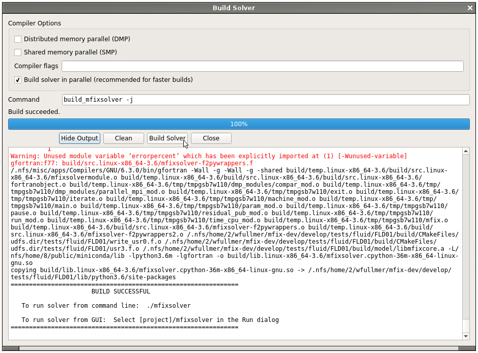
Before continuing to the Nodeworks panel, we first need to build a local mfixsolver so that the user defined functions (UDFs) get compiled into the code. Click on the Compile MFiX icon at the top and Build Solver on the pop up box. A serial solver is sufficient for this example. After the code builds successfully, switch to the Nodeworks interface (second panel on the bottom toolbar) to reveal a blank Nodeworks worksheet.

Now, add a Design of Experiments (DOE) node located in the Optimization Toolset collection of nodes. Next, we will work through the four tabs of the DOE node:

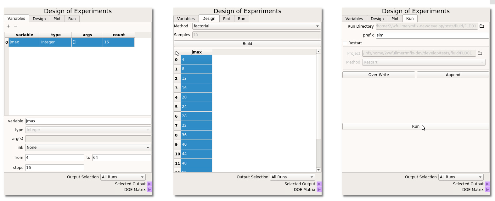
1. Variables In the first tab of the DOE node, click on the + icon (top left) to add a new variable to the table. Here, the MFiX input parameter that we would like to sweep is jmax, which takes no arguments, does not need to be linked to another variable (it will be our only variable in this example) and we will range jmax from 4 to 64 in 16 steps (step size of 4), as shown on the left below.
2. Design The second Design tab of the DOE is where we select the method to sample the design space. In this example, we will simply use factorial, i.e., uniform intervals, although other methods are available which are better suited to sweep higher-dimensional design spaces. Select factorial and click Build to generate the DOE table. We need to highlight the design points that we wish to run. Here, we want to run all cases in the design space. The entire table can be highlighted by clicking in the upper left corner as shown in the middle of the figure below.
3. Plot The plot of this 1-D factorial is uninteresting, but the Plot tab can be is very useful to visualize the sampling quality of higher dimensional spaces.
4. Run Finally, in the last tab of the DOE node we will generate the input files associated with this parameter sweep. Provide a prefix name for the run directories and click Over-Write to create the 16 directories, each with a different jmax corresponding to the DOE table. Click the Run button to launch the 16 jobs.

Warning

At the time of release 17.1, there is a known, minor issue with this case that the simulation does not terminate successfully after the code has completed. All simulations should complete in a short period of time. Run success can be probed by viewing the POST_* text files created by the UDFs.

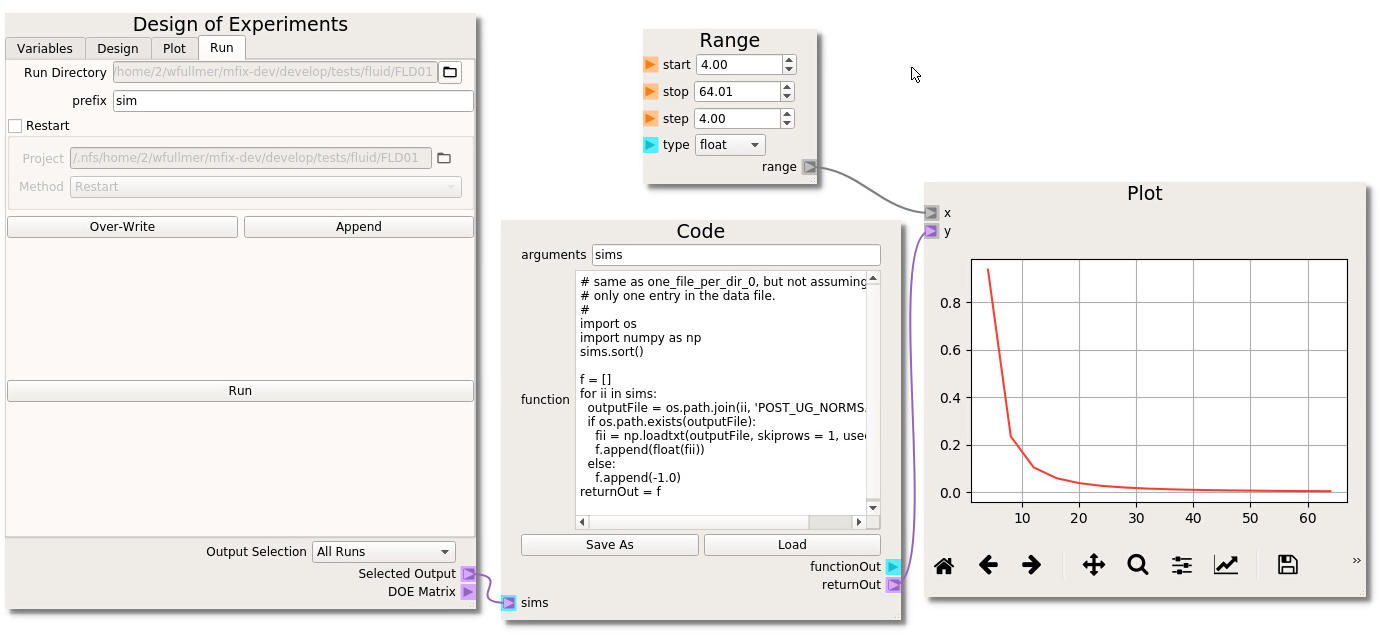
If you wish to visualize the results directly in the Nodeworks interface, we need to import the MFiX output data with a Code node. In this case, the UDFs create output files in each directory. An example code for this case is already available in the following section of this documentation. See the the Code Node Repo section to reproduce this code. Alternatively, the code can be imported directly: Open the Nodeworks documentation directly from the File menu under the Help tab; Navigate to the Code Node Repo tab; Click on the link to download the one_file_per_folder_1.txt example code; Back in the Nodeworks-MFiX interface, add a code node to the sheet; Click Load and find the one_file_per_folder_1.txt file in your local Downloads directory. We need to change the output file name from the generic data.txt to one of the UDF output file names. Here, we’ll look at the error between the computed velocity profile and the analytical solution which has been printed to POST_UG_NORMS.dat. These files have 3 header lines at the top, so we should set skiprows to 3 in the loadtxt command. Finally, three error outputs have been written (in columns 2-4) which can be accessed by setting the usecols flag to 1, 2, or 3 (first index is 0). We’ll use the L_1 norm which is stored the second column (usecols=1).

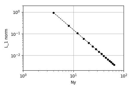
To plot the results, add a matplotlib Plot node, a numpy range to match the number of cells in each simulation. Make the connections as shown above and click the run icon to generate the plot. In the case of Poiseuille flow the velocity field develops into a parabolic profile and the convection term of the momentum equation vanishes. Therefore, the discretization error is determined entirely by the discretization of the of the viscous stress term, which, in MFIX, is second-order centered. By changing the settings of the plot (second icon from right), the results can be plotted in a log-log scale and verified to decay at a second order rate with respect to the number of transverse cells.

Ex. 2: Sensitivity Analysis for Single Particle Drop Test in MFIX GUI

The MFIX GUI incorporates the Nodeworks library into an integrated ‘Nodeworks’ mode. In this example, a single particle will be bounced in a simple DEM simulation. The setup for this example can be found in docs/source/data/particle_drop.zip . After unpacking the directory, the source files, the .mfx input file nodechart, and output data used in this example can be found.

The DOE node has additional features that are available when used in the Nodeworks tab of the MFIX GUI. This example will use MFiX keyword variables which can be searched in the keyword box. For this example, we will suppose that we do not know what is the major contributor to rebound height, but we will take an educated guess that particle-wall friction, particle diameter, particle-wall restitution coefficient, and particle-wall spring constant could have an effect. We then use all of these parameters within a DOE to investigate their effect and must run all the design points through MFIX. Range mew_w from 0.02 to 0.20, d_p0 from 0.0005 to 0.0015, des_en_wall_input from 0.7 to 0.9 and kn from 1000 to 10000.

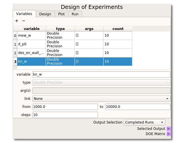
It is necessary to SELECT the points from the table that you wish to run by highlighting them. This is done because it is often desirable to oversample a design space and only run a fraction of the simulations to start. One can simply highlight all points by clicking in the upper left corner of the table.

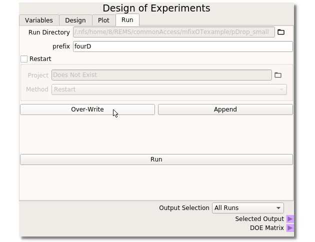
When used in the MFiX GUI, the DOE Node has a new MFiX tab that handles the creation of subdirectories and files for each run selected in the DOE tab. The run folder should be set automatically from the MFiX GUI. In this example ‘fourD’ is used as the Prefix to all subdirectory runs. This example uses a fresh run so no restart settings need be applied. Clicking the ‘Overwrite’ button will create/overwrite all subdirectories and necessary MFiX files to run the DOE through MFiX. When all options are set and the directories are created, clicking the ‘Run’ button will bring up the Run Solver dialogue box from the MFIX GUI to initiate the simulations. For the Output Selection, choosing All Runs will send the directory information out of the selected output terminal.

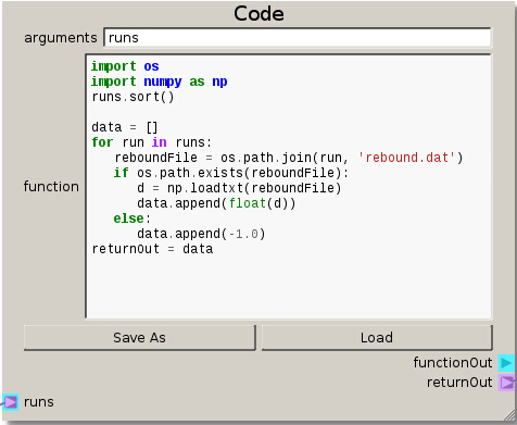
import os
import numpy as np
runs.sort()

data = []
for run in runs:
    reboundFile = os.path.join(run, 'rebound.dat')
    if os.path.exists(reboundFile):
        d = np.loadtxt(reboundFile)
        data.append(float(d))
    else:
        data.append(-1.0)
returnOut = data

The data of the DOE table is directed into the Code node by connecting the Selecting Output terminal (on the DOE node) to the runs terminal (on the Code node). With the code set up, the directories are sorted and looped over to read the data from the output files and passed on in a list. This output data will form the basis of the response surface.

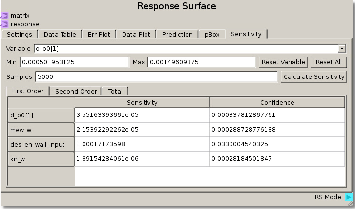
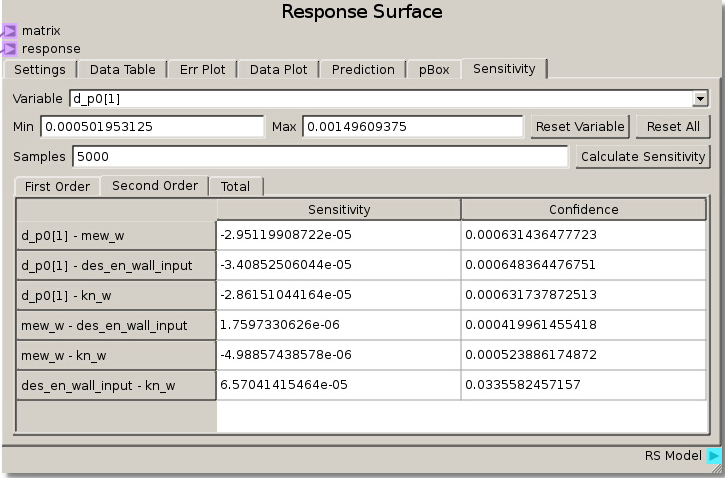
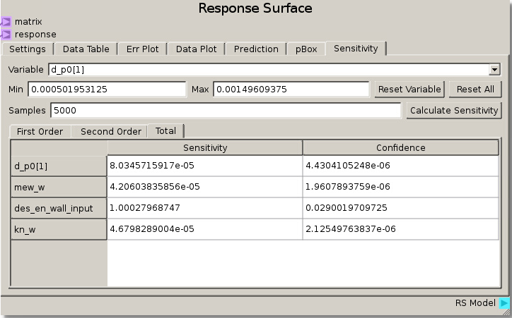
As in the previous example, the DOE Matrix output from the DOE node is fed into the matrix terminal and returnOut from the Code node is fed as the response into the Response Surface node. The default values for the Gaussian Process were used to fit a RSM. The sensitivity analysis reveals that the rebound height is almost exclusively sensitive to the particle-wall restitution coefficient as the total sensitivity of that variable was ~1.0. While this was a trivial example, it does illustrate how to tell which variables are important and which can be neglected. That is, we can glean that the system response does not depend on any variable but the particle-wall restitution coefficient and thus we have justification to eliminate all the other variables from further consideration as they are unimportant to our system.

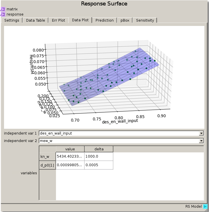
We can verify this finding again by placing des_en_wall_input as one of the independent variables in the Data Plot. Swapping the other variables through the other independent variable reveals that the response is unchanged which means they had no effect.

Ex. 3: Sensitivity Analysis of Multiple Particles in a Rotating Drum

The MFiX simulation in this example calculates the sliding angle of a group of particles in a rotating drum by slowly changing the direction of gravity and measuring when particles start to move past each other. A sensitivity analysis is performed between the four variables chosen to construct the Design of Experipments. It is hypothesized that one parameter will dominate the response while the others will have a small affect. This example has the same setup for the Design of Experiments node as the previous example, and the MFiX GUI simulation setup files can be found in docs/source/data/rotary_drum.zip . After unpacking the directory, the files necessary to include when building MFiX along with the .MFX data file and nodechart are available along with the raw data used later in subdirectories so that the simulation does not need to be run in order to continue this exercise.

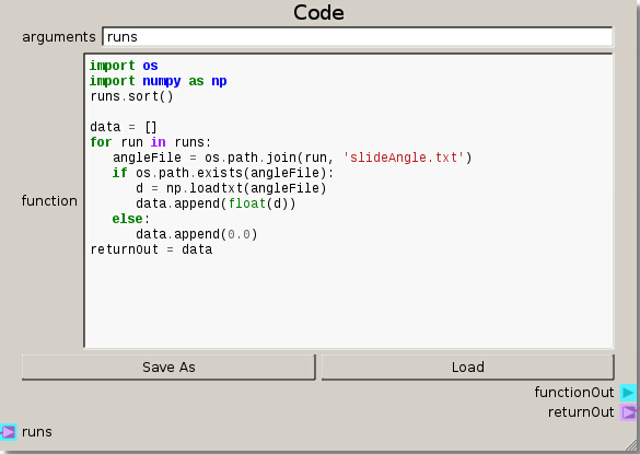
After constructing the DOE, setting up the file structure, and preparing the runs from the DOE node the Code node is modified to handle the output files for this case. The main difference in the code is now loading the slide angle data and appending a 0.0 for any missing data.

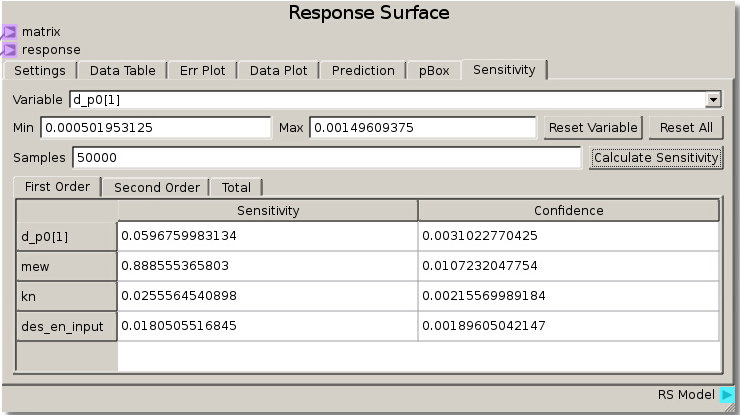
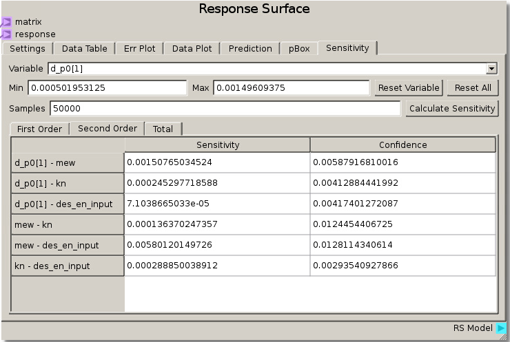
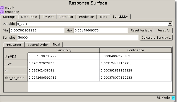
When the simulations have completed and the data has been run through the sheet, the RSM is set to use the Gaussian Process model with a nugget value set to 0.01 to fit the response values and minimize error. Calculating sensitivity in this case with 50000 samples reveals a high total sensitivity (~89%) to the coefficient of friction and lower sensitivity (less than ~10%) to the other 3 parameters. This tells us that the angle at which particles begin to move past one another is highly dependent on the coefficient of friction parameter.

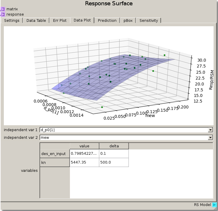
Looking at hypersurfaces placing the coefficient of friction as one of the independent variables reveals a high dependence on coefficient of friction with minor deviations due to the very low sensitivity of the other parameters.

Extension: Over fitting Data

When choosing parameters for the Gaussian Process RSM it is important to take note of both how well the model fits the data (minimizing error) and noise tolerance. Using Extension 8 as a base for comparison, let us explore this concept of over fitting by utilizing the Err Plot capabilities in the Response Surface node.

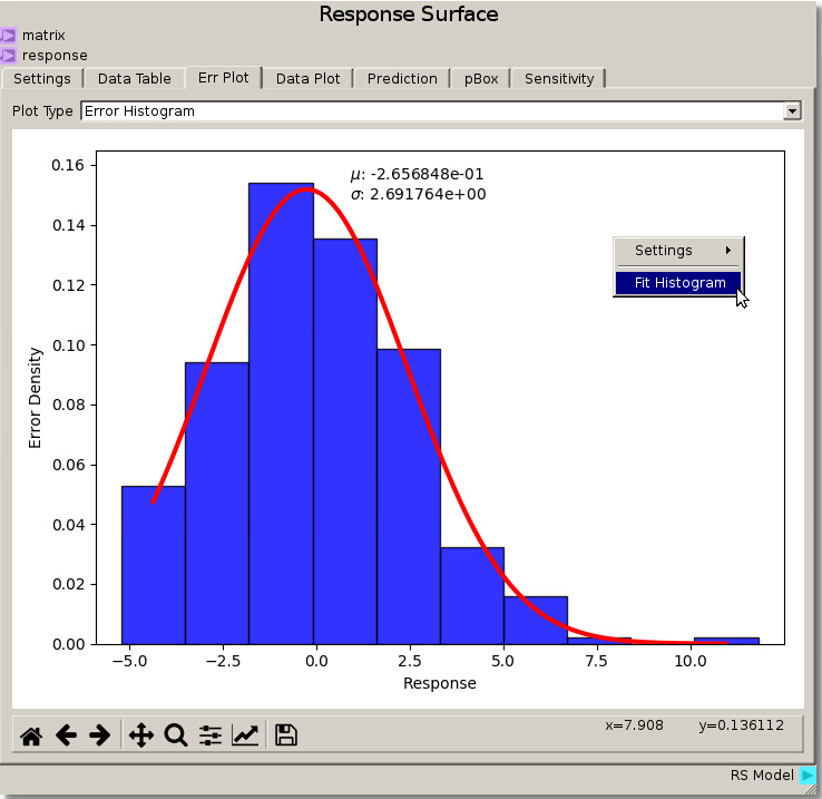
Changing the Err Plot tab Plot Type from Parity Plot to Error Histogram generates an Error Density Histogram between the Response and the data that was fit. Right-clicking and selecting Fit Histogram will fit a distribution to the histogram and display the mean and standard deviation. From here we can see from utilizing the Gaussian Process fit with a nugget value of 0.01 gives an error distribution with mean ~ -0.266 and deviation ~ 2.7. The Response Surface Data Plot from above displays a smooth response amongst the fitted data.

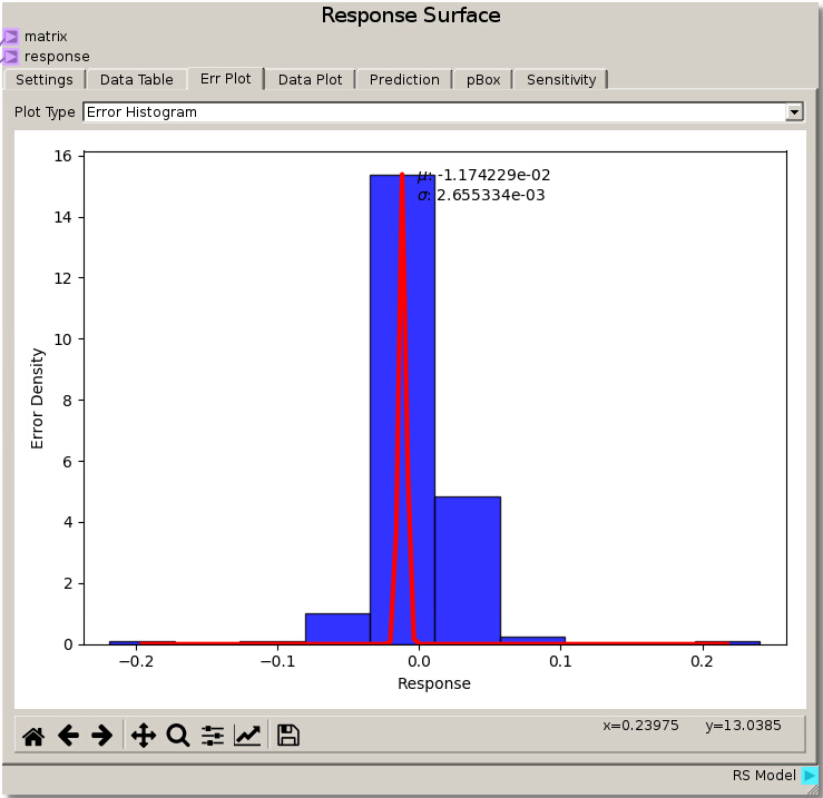
Modifying the Gaussian Process nugget to 0.001 and refitting gives a much tighter error distribution with mean ~ -0.0117 and deviation ~ 0.002655 which reduced the error and the spread of the error versus the previous parameters. However, viewing the Data Plot reveals a warped surface, showing how the Response Surface is attempting to match every data point as the Gaussian Process minimizes the error. This is an example of over fitting the data where the model tries to capture all the noise that would normally be present in experimental variations and representing it as true value rather than a smooth average with noise variance.

Example 4: MFiX Optimization of a Continuous Flow Fluidized Bed

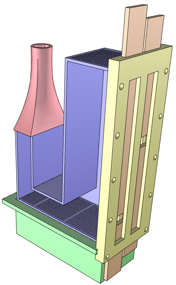
This example will find the optimum inlet flow rates to achieve separation of two different particles in a continuously flowing fluid bed. The standpipe is filled with heavier, larger particles and smaller, lighter particles that will flow through a connecting L-valve into the bed region. The aim is to separate the particles by having the heavier particles leave the system through a lower exit and the lighter particles through an upper exit by adjusting the gas inlet flow rate in the L-valve section and in the fluid bed region. The setup for this example can be found in docs/source/data/continuous_flow.zip . After unpacking the directory, the source files, the .mfx input file nodechart, and output data used in this example can be found.

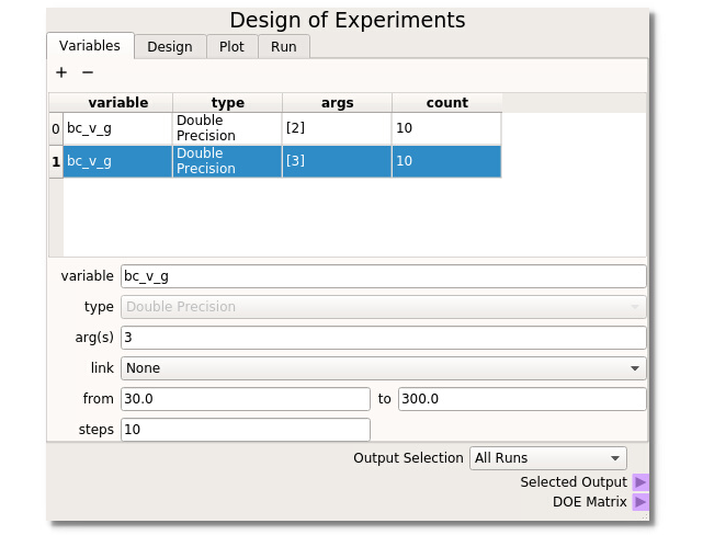
For this example the Design of Experiments is set up with bc_v_g(2) (gas flow in the L-valve portion) ranging from 25.0 to 250.0 cm/s and bc_v_g(3) (the gas flow for the bed region) ranging from 10 to 300 cm/s, both taking 10 steps. With the DOE built, runs selected, and directories created the MFiX simulations can be run.

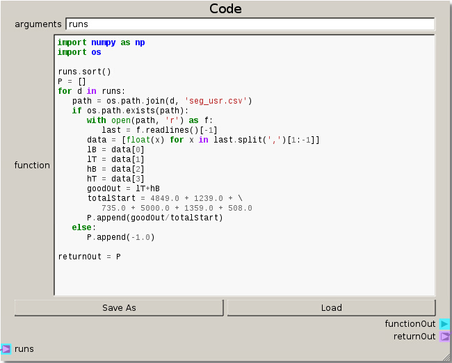
This setup for the Code node reads in the simulation data stored in ‘seg_usr.csv’(written out of a custom MFiX UDF) to create a single output response. The objective is to get the highest ratio of desired particles out of their respective exits. This is quantified by looking at the ratio of the number of light particles exiting the top and the heavy particles leaving the bottom to the initial total number of particles in the system at the start.

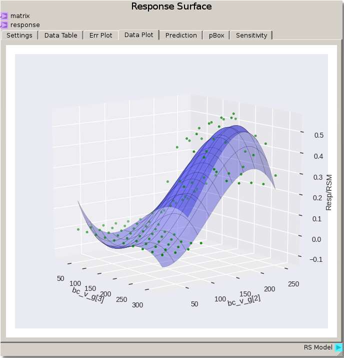
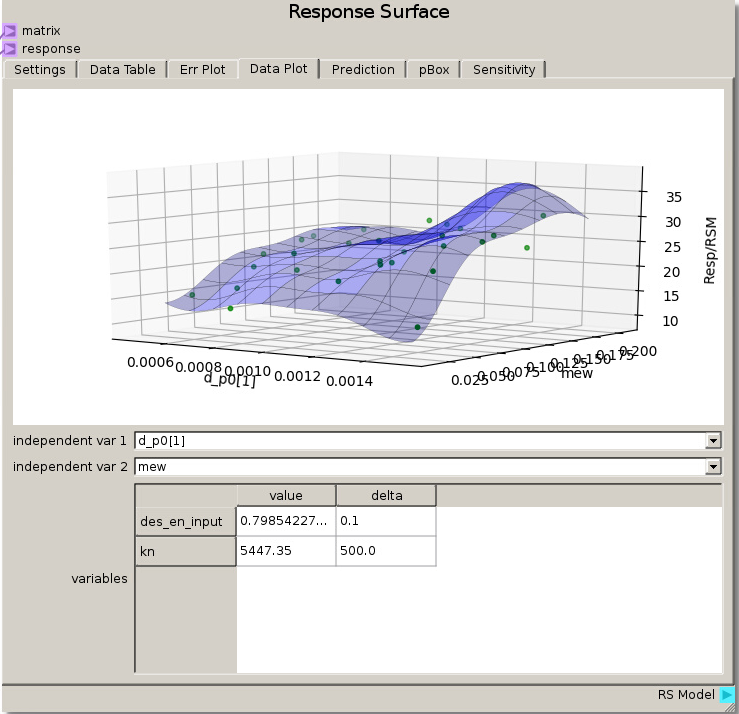
Instead of viewing each case individually, we can do a quick initial evaluation of the data by viewing the Data Plot of the Response Surface node using the default settings for a 3rd order polynomial fit. From this view we see multiple instances of 0.0 value for the response. This is due to the velocity of those cases being too low to allow the particles to move and become fluidized so that no particles actually become separated.

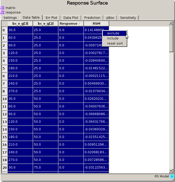
The simplest way to remove seemingly irrelevant (non-separating) runs is to highlight and exclude the 0.0 Response values after sorting the Response column by clicking on the column header. This can also be used to exclude values from run that were incomplete or have response values above 1.0, showing an issue with the separation ratio.

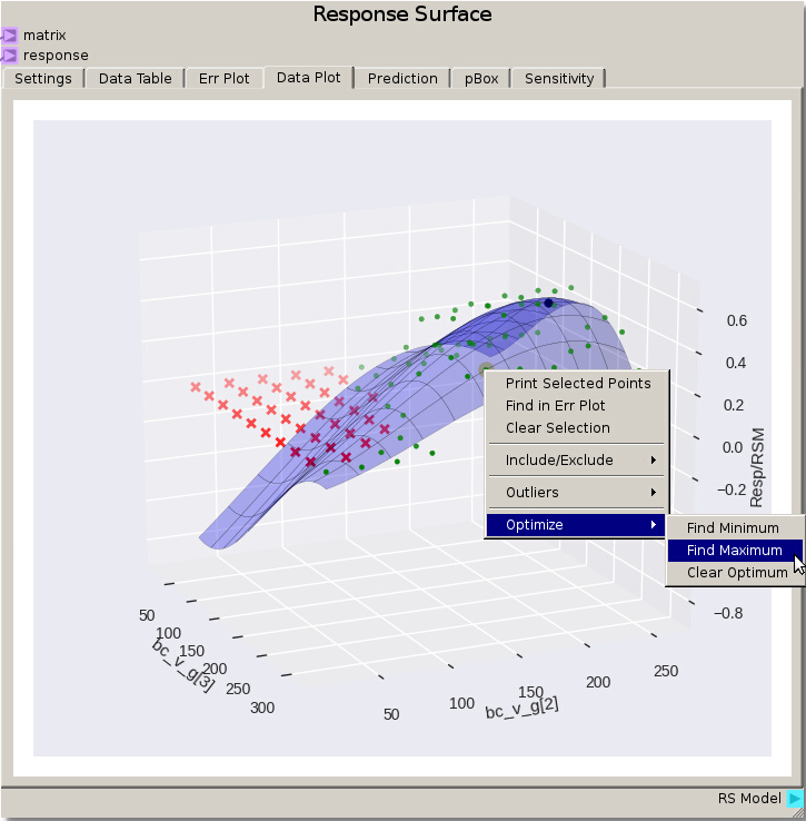
After refitting the same 3rd degree polynomial with points excluded an optimal region appears and an optimal point to the response surface can be found by right clicking and selecting Optimize -> Find Maximum from the menu. For this fit the optimum point is around 215 cm/s for bc_v_g [2] and 220 cm/s for bc_v_g [3]. Refitting with the default Gaussian Process model values gives an optimum around 184 cm/s for bc_v_g [2] and 201 cm/s for bc_v_g[3]. Remember there are several options for reducing error such as adjusting the model fit parameters, excluding different data points (such as values below say 20% separation), and refining the DOE around the region of interest and running the MFiX simulations again.