Ex. 4: Uncertainty Quantification
In this example, we will demonstrate the use of the surrogate modeling strategy for forward propagating a set of model input uncertainties into model output uncertainty. We will use a simple function as the full model, the Ishigami Function
Build the Surrogate
In this section, we’ll build a surrogate model of the Ishigami function which will be used for forward propagation of hypothetical input uncertainties.
Click on the
to launch the wizard–we’ll use many of the wizard defaults to do most of the work setting up the surrogate model for the Ishigami function.
Click on the
Forward Propagationtab and set theFunction to be analyzedtoIshigamiand theMethodtosurrogate. TheNumber of dimensionsshould not be de-selected and constrained to3.Click
Populate NodesIn the
Design of Experimentsnode, click on theDesigntab and set the samplingMethodtohaltonand clickBuild. The sampling design can be visualized in thePlottab and saved if desired.In the
Response Surfacenode, click on theModeltab and set theCross validation pointsto 0. Next check and highlight thegaussian processresponse surface model and reduce thenuggetone order of magnitude to1e-06. The rest of the surrogate modeling defaults are sufficient for this example, but the user is certainly welcome to build a different, possibly better surrogate of the Ishigami function.Before constructing the surrogate, navigate to the
Forward Propagationnode and set the Aleatory and Epistemic samples to low values, e.g., 3 each. We’ll define and propagate the input uncertainties after construction of the surrogate.Press
and voilà a gaussian process surrogate model of the Ishigami function is constructed.
The model can be viewed in the Plot tab of the Response Surface node. The
error plot should show local errors within +/- 0.01. Quantitatively, the surrogate
should have \(L_1\), \(L_2\), and \(L_\infty\) norms of 4.1e-04, 4.5e-4
and 6.2e-4, respectively.
Forward Propagation
In this section, we’ll select some hypothetical input uncertainties and propagate them through the previously constructed surrogate model.
Select the
ainput variable from the table. Let’s consideraan aleatoryVariable Typehaving a normalDistributionwith aMeanof -1.0 and aStandard Deviationof 0.3.Select
bfrom the table and give it the same properties asabut with aMeanof +1.0.To test the mixed-UQ method, let’s make
can epistemicVariable TyperangingFrom-1To+1.Make sure that the
Epistemic Methodabove the table is set to latin hypercube.With these settings, we can see from the example distribution function plots that sampling outside bounds will be a very low probability event. Therefore, we can simply re-draw the
Samples outside rangefor this case.Select a number of
Aleatory samplesandEpistemic samplesFinally, click
Calculate Propagationto forward propagate the designed input uncertainty into an output uncertainty.
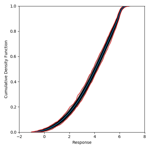
For the selected input uncertainties, we find that the output uncertainty is dominated
by the two aleatory uncertainties. This may not be so surprising given that the coefficient
of the third input variable in the Ishigami function is almost two orders of magnitude
lower than the second. Therefore, the size of the p-box will shrink with an increasing
number of aleatory samples. For 1000 Aleatory samples and 200 Epistemic samples
we find that the 95th-percentile occurs at response between 5.94 to 6.12. The resultant
p-box for this case is provided below. Note that the exact same values may not be recovered
when repeating this example due to the random nature of the propagation sampling.
Verification
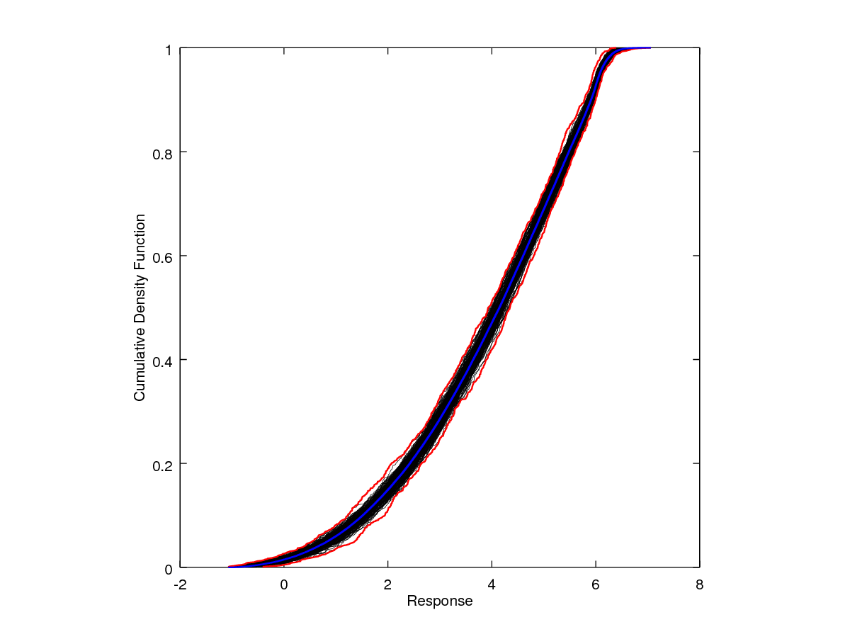
In practice, the model being replaced with a surrogate is expensive and, thus, direct sampling of the full model to forward propagate the input uncertainty is not possible. It is, however, for this simple demonstration problem. To validate Nodework’s forward propagation procedure, the previous example problem has been coded into a simple Matlab or Octave script which is provided below. Running the script in one instance resulted in the p-box generated above. Qualitatively, the output response propagated through the surrogate is very to the analogous output uncertainty propagated directly through the full model. Quantitatively, we can see some slight discrepancies. Again, considering the 95th-percentile as the decision quantity, the direct p-box gives a response range of 5.9490 to 6.1417, slightly higher than reported from the surrogate constructed p-box. Of course, some of the discrepancy is just due to the randomization of sampling. However, reconstructing both the script (direct) and Nodeworks (surrogate) p-boxes several times shows that the surrogate, while very close, tends to give slightly lower responses at the 95th-percentile.
%
% Ishigami function:
% r = sin(x1) + a*sin(x2)^2 + b*x3^4*sin(x1);
%
% Ref: see https://www.sfu.ca/~ssurjano/ishigami.html and refs therein.
%
clear all
close all
clc
%
% model constants
a = 7.0;
b = 0.1;
%
% input uncertainty properties for forward propagation UQ
x1o    = -1.0;
sigma1 = 0.3;
x2o    = 1.0;
sigma2 = 0.3;
x3a    = -1.0;
x3b    = 1.0;
%
% Num. of aleatory and epistemic samples
Na = 1000;
Ne = 200;
%
% direct sample the Ishigami function
r  = zeros(Na,Ne);
for jj = 1:Ne
    delx3 = (x3b - x3a)/double(Ne);
    x3 = x3a + double(jj - 1)*delx3 + rand(1)*delx3;
    for ii = 1:Na
        x1 = x1o + sigma1*randn;
        x2 = x2o + sigma2*randn;
        r(ii,jj) = sin(x1) + a*sin(x2)^2 + b*x3^4*sin(x1);
    end
end
%
% plot p-box
grey = [0.5 0.5 0.5];
p = linspace(1.0/double(Na),1.0,Na)';
figure;
hold on;
%
% sort each CDF and plot
rs = sort(r);
for jj = 1:Ne
    plot(rs(:,jj),p,'-k', 'LineWidth', 0.2);
end
%
% highlight the p-box
pboxL = zeros(Na,1);
pboxR = zeros(Na,1);
for ii = 1:Na
    pboxL(ii,1) = min(rs(ii,:));
    pboxR(ii,1) = max(rs(ii,:));
end
plot(pboxL,p,'-r', 'LineWidth', 1.);
plot(pboxR,p,'-r', 'LineWidth', 1.);
%
% sort single CDF
rall = zeros(Na*Ne,1);
for jj = 1:Ne
    ij = (jj-1)*Na;
    rall(ij+1:ij+Na) = r(:,jj);
end
rall = sort(rall);
pall = linspace(1.0/double(Na*Ne),1.0,Na*Ne)';
plot(rall,pall,'-b', 'LineWidth', 1.);
%
% label axes and save
xlabel('Response');
ylabel('Cumulative Density Function');
print -dpng ishigami_pbox.png
%
% write out the 95%
msg = "\n\n The 95%% p-box range is:\t %12.4e \t to\t %12.4e \n";
tmp1 = pboxL(floor(0.95*Na));
tmp2 = pboxR(floor(0.95*Na));
printf(msg,tmp1,tmp2);
%
% exit if run in batch mode
%exit;
%
% EOF eof eor EOR