7. Analytical solution for particle-settling in fluid

An analytical expression can be obtained for the velocity of kinematic shocks (also referred to as concentration shocks). Two shock fronts develop in a settling system as depicted in Fig. 7.1. One of the shocks propagates in the direction of gravity (downward), while the other is aligned with the direction of packing (upward).

Fig. 7.1 Schematic showing the settling problem.

Settling is governed by the balance between drag, gravity, and buoyancy. Consider the two-fluid model (TFM) system of equations. The phasic continuity equations are given by,

(7.1) $$\frac{\partial}{\partial t}\rho_{g} \epsilon_{g} + \frac{\partial}{\partial x_{i}} (\rho_{g} \epsilon_{g} u_{gj}) = R_{g}$$

(7.2) $$\frac{\partial}{\partial t}\rho_{s} \epsilon_{s} + \frac{\partial}{\partial x_{i}} (\rho_{s} \epsilon_{s} u_{sj}) = R_{s}$$

where, $\rho_{g},\epsilon_{g},u_{gj},R_{g}$ represent density, volume fraction, $j^{th}$ component of velocity and mass source term of the gas-phase respectively. The corresponding terms in the solid phase continuity equations are represented with the subscript $s$. The phasic momentum equations are given by,

(7.3) $$\frac{\partial}{\partial t}(\rho_{g} \epsilon_{g} u_{gi}) + \frac{\partial}{\partial x_{i}} (\rho_{g} \epsilon_{g} u_{gi} u_{gj}) = -\epsilon_{g} \frac{\partial P_{g}}{\partial x_{i}} + \frac{\partial}{\partial x_{i}} (\epsilon_{g} \tau_{gij}) + \beta (u_{si} - u_{gi}) + \rho_g \epsilon_{g} g_{i} + S_{gi}$$

(7.4) $$\frac{\partial}{\partial t}(\rho_{s} \epsilon_{s} u_{si}) + \frac{\partial}{\partial x_{i}} (\rho_{s} \epsilon_{s} u_{si} u_{sj}) = -\epsilon_{s} \frac{\partial P_{g}}{\partial x_{i}} + \frac{\partial}{\partial x_{i}} (\epsilon_{s} \tau_{sij}) + \beta (u_{gi} - u_{si}) + \rho_s \epsilon_{s} g_{i} + S_{si}$$

$P_{g},\tau_{gij},S_{gi}$ represent pressure, shear stress and source term in the gas phase. $\tau_{sij}$ contains contributions from inter-particle collisions and $S_{si}$ represents the momentum source term in the solids phase. The following assumptions are made for the settling problem.

1. One-dimensional system

2. Shear stress terms are negligible

3. Particle-particle and particle-wall interactions are negligible

4. Isothermal with no phase change

5. Both the phases are incompressible

Based on these assumptions, the continuity equations Eq.7.1, Eq.7.2 can be combined to give,

(7.5) $$\frac{\partial}{\partial x} (\epsilon_{g} u_{g}) + \frac{\partial}{\partial x} (\epsilon_{s} u_{s}) = \frac{\partial j}{\partial x} = 0$$

The notation for velocity components is dropped since one-dimensional analysis is used. It is seen that the volumetric flux, $j$ is a constant for the problem considered. The momentum equations Eq.7.3, Eq.7.4 can be simplified to give,

(7.6) $$-\frac{\partial P_{g}}{\partial x} + \frac{\beta}{\epsilon_{g}} u_{r} + \rho_{g} g = 0$$

(7.7) $$-\frac{\partial P_{g}}{\partial x} - \frac{\beta}{\epsilon_{s}} u_{r} + \rho_{s} g = 0$$

where, $u_{r} = u_{s} - u_{g}$ is the relative velocity. Subtracting Eq.7.7 from Eq.7.6 gives a relation between the relative velocity, drag function $\beta$ and acceleration due to gravity as follows,

(7.8) $$u_{r} = \frac{g \Delta \rho}{\beta} \epsilon_{g} \epsilon_{s}$$

where, $\Delta \rho = \rho_{s} - \rho_{g}$. The drag function , $\beta$ is given by,

(7.9) $$\beta = \frac{3}{4} \frac{\rho_{g} \epsilon_{g} \epsilon_{s} C_{D} u_{r}}{d_{p}} \epsilon_{g}^{-2.65}$$

The drag coefficient for Stokes’ law follows,

(7.10) $$C_{D} = \frac{24}{Re} = \frac{24 \mu_{g}}{\rho_{g} u_{r} d_{p} \epsilon_{g}}$$

The final expression for relative velocity considering Stokes’ drag law is given by,

(7.11) $$u_{r} = \frac{g \Delta \rho d_{p}^{2}}{18 \mu_{g}} \epsilon_{g}^{3.65}$$

The laboratory and travelling frame of references are depicted in Fig. 7.2. The quantities are related as follows:

(7.12) $$\begin{split}u_{gA}^{'} =& u_{gA} + u_{shock}, \\ u_{gB}^{'} =& u_{gB} + u_{shock}, \\ u_{sA}^{'} =& u_{sA} + u_{shock}, \\ u_{sB}^{'} =& u_{sB} + u_{shock}\end{split}$$

The variables with $'$ denote the travelling frame of reference. The phasic volumetric fluxes are related by,

(7.13) $$\begin{split}j_{gA}^{'} =& j_{gA} + \epsilon_{gA} u_{shock}, \\ j_{gB}^{'} =& j_{gB} + \epsilon_{gB} u_{shock}, \\ j_{sA}^{'} =& j_{sA} + \epsilon_{sA} u_{shock}, \\ j_{sB}^{'} =& j_{sB} + \epsilon_{sB} u_{shock}\end{split}$$

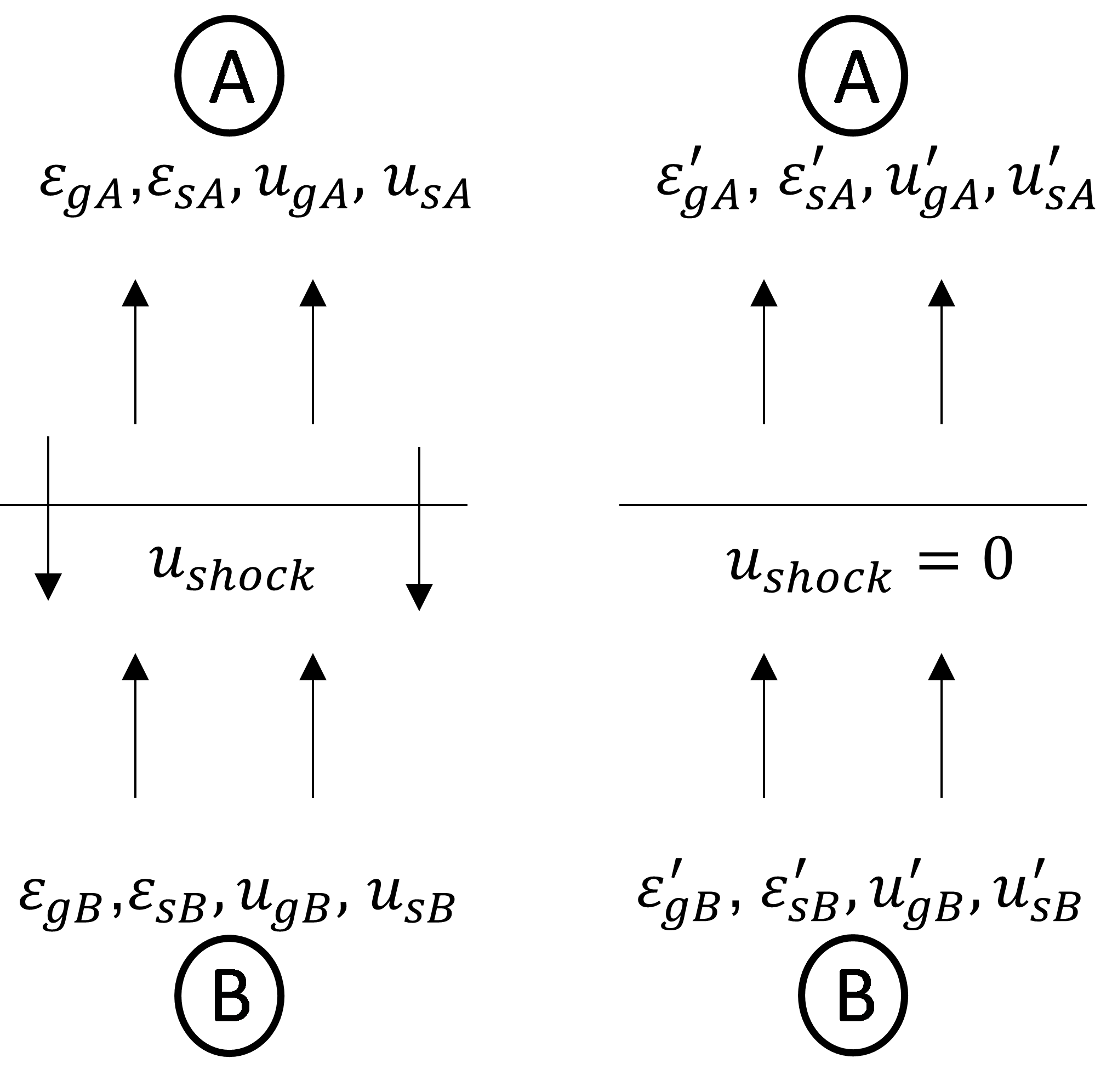
Fig. 7.2 Laboratory (left) and traveling (right) frame of references for the kinematic shock wave.

Since there is no exchange of mass before and after the kinematic shock, additional constraints are obtained as follows,

(7.14) $$\begin{split}j_{gA}^{'} =& j_{gB}^{'}, \\ j_{sA}^{'} =& j_{sB}^{'}\end{split}$$

Simplifying Eq.7.12, Eq.7.13, Eq.7.14, the shock velocity is obtained as,

(7.15) $$u_{shock} = -\frac{j_{sB}-j_{sA}}{\epsilon_{sB} - \epsilon_{sA}}$$

The phasic volumetric flux, $j$ is related to the total volumetric flux and drift flux [33] as follows,

(7.16) $$j_{s} = \epsilon_{s} j + j_{gs}$$

where, the drift flux, $j_{gs}$ is related to the relative velocity [33] given by,

(7.17) $$j_{gs} = \epsilon_{s} (u_{s} - j) = \epsilon_{s} \epsilon_{g} u_{r}$$

Upon further simplification of Eq.7.15 using Eq.7.16 and Eq.7.17, the analytical expression for shock velocity is obtained as follows,

(7.18) $$u_{shock} = -\Big( j + \frac{(\epsilon_{s} \epsilon_{g} u_{r})_{B} - (\epsilon_{s} \epsilon_{g} u_{r})_{A}}{\epsilon_{sB} - \epsilon_{sA}} \Big)$$

where, $u_{r}$ is given by Eq.7.11.