Particle distributions

MFIX-Exa can generate constant (monodisperse or single-sized) particles or polydisperse particles that follow a normal, log-normal, or uniform distribution. A user-defined custom distribution can be specified by providing discrete probabilities via a text input file.

In addition to the distribution type, the distribution weighting must be specified; MFIX-Exa supports two distribution weightings:

Number-weighted diameter distribution

The number-weighted diameter density function, \(f_X^N(x)\,dx\), can be interpreted as defining the number of particles with diameters between \(x\) and \(x+dx\), divided by the total number of particles.

Volume-weighted diameter distribution

The volume-weighted diameter density function, \(f_X^V(x)\,dx\), similarly can be interpreted as defining the volume of particles with diameters between \(x\) and \(x+dx\), divided by the total volume of particles.

Warning

Number-weighted and volume-weighted distributions are not interchangeable. Failing to specify the correct distribution weighting can result in unexpected behavior.

The code uses both distribution weightings, computing (or approximating) whichever distribution weighting that was not provided. For example, if a number-weighted normal distribution is provided, the corresponding volume-weighted normal distribution is computed. The volume-weighted distribution is used to calculate the number of particles (or parcels) to generate in an initial condition region. The number-weighted distribution is sampled when DEM particles are created, while the volume-weighted distribution is sampled when creating PIC parcels. Sampling the volume-weighted distribution for PIC parcels allows for fewer parcels to represent very small particles while using more parcels to represent large particles in the distribution. The statistical weight of the parcels is adjusted so that the number-distribution is represented accurately.

The following sections overview the distributions supported by MFIX-Exa and the input parameters that control their behavior.

constant distribution

The constant distribution defines a monodisperse (single-valued) distribution and uses the following inputs:

	Description	Type	Default
constant	size of the mono-disperse distribution	Real	N/A

In the following example, a cuboid is filled with 1 mm diameter monodisperse particles with 2500 kg·m^-3 density. The initial condition region volume is 0.001 m³, and it has a solids volume fraction of 0.05 (5% solids).

Listing 10 Snippet of inputs defining a constant distribution. This is not a complete input file.

# Regions for defining ICs and BCs
# -----------------------------------------------------------------------
mfix.regions = full-domain

regions.full-domain.lo  = 0.0  0.0  0.0
regions.full-domain.hi  = 0.1  0.1  0.1

# Initial Conditions
# -----------------------------------------------------------------------
ic.regions = full-domain

mfix.particle_init_type = Auto

# Full domain
#~~~~~~~~~~~~~~~~~~~~~~~~~~~~~~~~~~~~~~~~~~~~~~~~~~~~~~~~~~~~~~~~~>
ic.full-domain.fluid.volfrac  = 0.95

ic.full-domain.fluid.density  = 1.0
ic.full-domain.fluid.pressure = 0.0
ic.full-domain.fluid.velocity = 0.0  0.0  0.0

ic.full-domain.solids  = solid0

ic.full-domain.packing = random

ic.full-domain.solid0.volfrac   = 0.05
ic.full-domain.solid0.velocity  = 0.00  0.00  0.00

ic.full-domain.solid0.diameter = constant
ic.full-domain.solid0.diameter.constant = 1000.e-6  # (m)

ic.full-domain.solid0.density =  constant
ic.full-domain.solid0.density.constant  = 2500.0    # (kg/m^3)

An MFIX-Exa DEM simulation generates approximately 95,500 particles, while a PIC simulation with pic.close_pack = 0.64, pic.parcels_per_cell_at_pack = 64, and an Eulerian mesh spacing \(\Delta x\) of 3.125 mm generates approximately 164,000 parcels.

normal distribution

The normal or Gaussian distribution is given by

(1)\[f_X(x) = \frac{d}{dx}F_X(x) = \frac{1}{\sigma \sqrt{2\pi}} \exp{\left(- \frac{(x - \mu)^2 }{ 2 \sigma^2 }\right)}\]

where the parameter \(\mu\) is the distribution mean, and \(\sigma\) is the standard deviation. The inputs used to specify the distribution are provided in the following table.

	Description	Type	Default
type	distribution weighting: number-weighted or volume-weighted	string	N/A
mean	mean of the normal random variable, \(X\)	Real	N/A
std	standard deviation of the normal random variable, \(X\)	Real	N/A
min	Minimum particle diameter. Drawn samples below min are discarded and a new sample is drawn.	Real	N/A
max	Maximum particle diameter. Drawn samples above max are discarded and a new sample is drawn.	Real	N/A
bins	Number of bins used when discretizing the distribution to approximate the number of particles within an initial condition region.	int	64

In the following example, a cuboid with volume 0.001 m³ is filled with a number-weighted normal distribution with 1 mm mean diameter and 0.25 mm standard deviation. The minimum and maximum particle diameters are 0.25 mm and 1.75 mm, respectively.

Listing 11 Snippet of inputs defining a number-weighted normal distribution. This is not a complete input file.

# Regions for defining ICs and BCs
# -----------------------------------------------------------------------
mfix.regions = full-domain

regions.full-domain.lo  = 0.0  0.0  0.0
regions.full-domain.hi  = 0.1  0.1  0.1

# Initial Conditions
# -----------------------------------------------------------------------
ic.regions = full-domain

mfix.particle_init_type = Auto

# Full domain
#~~~~~~~~~~~~~~~~~~~~~~~~~~~~~~~~~~~~~~~~~~~~~~~~~~~~~~~~~~~~~~~~~>
ic.full-domain.fluid.volfrac  = 0.95

ic.full-domain.fluid.density  = 1.0
ic.full-domain.fluid.pressure = 0.0
ic.full-domain.fluid.velocity = 0.0  0.0  0.0

ic.full-domain.solids  = solid0

ic.full-domain.packing = random

ic.full-domain.solid0.volfrac   = 0.05
ic.full-domain.solid0.velocity  = 0.00  0.00  0.00

ic.full-domain.solid0.diameter = normal
ic.full-domain.solid0.diameter.type = number-weighted
ic.full-domain.solid0.diameter.mean = 1000.e-6  # (m)
ic.full-domain.solid0.diameter.std  =  250.e-6  # (m)
ic.full-domain.solid0.diameter.min  =  250.e-6  # (m)
ic.full-domain.solid0.diameter.max  = 1750.e-6  # (m)

ic.full-domain.solid0.density =  constant
ic.full-domain.solid0.density.constant  = 2500.0 # (kg/m^3)

An MFIX-Exa DEM simulation with these settings generates approximately 81,700 particles. The particle size distribution is shown in Fig. 9 (open circles) in addition to the number-weighted (orange) and volume-weighted (blue) density functions. As noted by Weiner [Wei11], the volume-weighted probability density function (PDF) is shifted to the right of the number-weighted PDF.

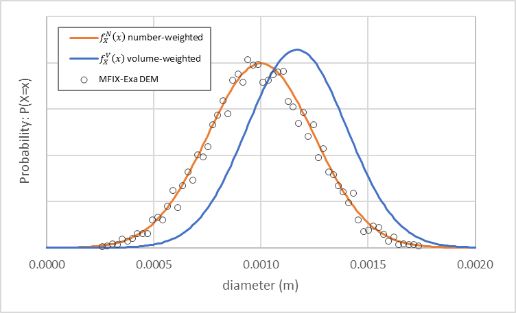
Fig. 9 MFIX-Exa DEM particle size distribution (open circles) generated from example inputs. The number-weighted density function (orange) with 1 mm mean and 0.25 mm standard deviation, and volume-weighted density function with ~1.17 mm mean and ~0.23 mm standard deviation are also plotted.

An MFIX-Exa PIC simulation with the same settings generates approximately 82,000 parcels when pic.close_pack = 0.64, pic.parcels_per_cell_at_pack = 32, and the Eulerian mesh spacing \(\Delta x\) is 3.125 mm. The parcel size distribution shown in Fig. 10 (open triangles) follows the volume-weighted density function. Small closed circles illustrate the effective particle size distribution, computed by multiplying each observation by the parcel statistical weight. For example, if a parcel has statistical weight of 10, then 10 observations are recorded in the bin capturing the parcel’s diameter.

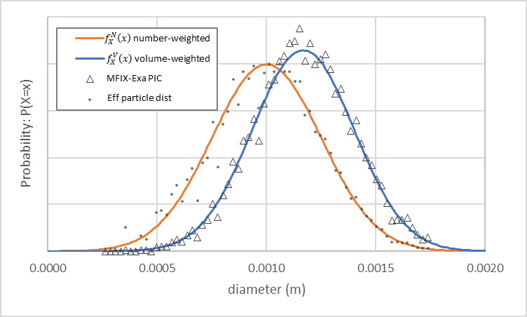
Fig. 10 MFIX-Exa PIC parcel size distribution (open triangles) generated from example inputs. The number-weighted density function (orange) with 1 mm mean and 0.25 mm standard deviation, and volume-weighted density function (blue) with ~1.17 mm mean and ~0.23 mm standard deviation are also plotted.

The following sections outline how MFIX-Exa computes volume-weighted normal density function parameters from number-weighted normal density function parameters, and conversely, how number-weighted normal density function parameters are computed from volume-weighted density function parameters.

Computing volume-weighted normal density function parameters, \(\mu_V\) and \(\sigma_V\), from number-weighted normal density function parameters, \(\mu_N\) and \(\sigma_N\)

The volume-weighted density function, \(f_X^V(x)\), computed from the normally distributed number-weighted density function, \(f_X^N(x)\), is normally distributed with mean, \(\mu_V\), and variance, \(\sigma_V^2\). An expression for the volume-weighted density function is obtained by multiplying (1) by \(x^3\) and substituting in the mean and standard deviation of the number-weighted distribution.

\[\tilde{f}_X^V(x) = \frac{x^3}{\sigma_N \sqrt{2\pi}} \exp{\left(- \frac{(x - \mu_N)^2 }{ 2 \sigma_N^2 }\right)}\]

The mean of this distribution is computed as

(2)\[\begin{split}\begin{align} \mu_V =& \frac{ \int_{-\infty}^{\infty} x \tilde{f}_X^V(x) dx }{\int_{-\infty}^{\infty} \tilde{f}_X^V(x) dx } \\[10pt] =& \frac{3\sigma_N^4 + 6\sigma_N^2\mu_N^2 + \mu_N^4}{3\sigma_N^2 \mu_N + \mu_N^3} \end{align}\end{split}\]

and the variance is given by

(3)\[\begin{split}\begin{align} \sigma^2_V =& \frac{ \int_{-\infty}^{\infty} (x - \mu_V)^2 \tilde{f}_X^V(x) dx }{\int_{-\infty}^{\infty} \tilde{f}_X^V(x) dx } \\[10pt] =& \frac{3\sigma_N^4 (3\mu_N + 2b) + \sigma^2(\mu_N^3 + 6\mu_N^2 b + 3\mu_Nb^2)+\mu_N^3 b^2}{3\sigma_N^2 \mu_N + \mu_N^3} \end{align}\end{split}\]

where \(b = (\mu_N - \mu_V)\). Because the volume-weighted distribution is normally distributed, the computed mean and variance can be substituted directly into (1).

\[f_X^V(x) = \frac{1}{\sigma_V \sqrt{2\pi}} \exp{\left(- \frac{(x - \mu_V)^2 }{ 2 \sigma_V^2 }\right)}\]

Computing number-weighted normal density function parameters, \(\mu_N\) and \(\sigma_N\), from volume-weighted normal density function parameters, \(\mu_V\) and \(\sigma_V\)

The number-weighted density function mean and standard deviation, \(\mu_N\) and \(\sigma_N\), are computed from the volume-weighted mean and standard deviation, \(\mu_V\) and \(\sigma_V\), by solving the nonlinear system of equations constructed from (2) and (3) for \(\mu_N\) and \(\sigma_N\).

\[\begin{split}\begin{align} f_1(\mu_N,\sigma_N) &= \left( 3\sigma_N^4 + 6\sigma_N^2\mu_N^2 + \mu_N^4 \right) - \mu_V \left( 3\sigma_N^2 \mu_N + \mu_N^3 \right) = 0 \\ f_2(\mu_N,\sigma_N) &= \left(3\sigma_N^4 (3\mu_N + 2b) + \sigma^2(\mu_N^3 + 6\mu_N^2 b + 3\mu_Nb^2)+\mu_N^3 b^2\right) - \sigma^2_V \left( 3\sigma_N^2 \mu_N + \mu_N^3 \right) = 0 \end{align}\end{split}\]

This system is solved using the homotopy method outlined in Burden and Faires [BF10]. To ensure rapid convergence, initial guesses for \(\mu_N\) and \(\sigma_N\) are calculated from the density function created by dividing (1) by \(x^3\) and substituting in the mean and standard deviation of the volume-weighted distribution, \(\mu_V\) and \(\sigma_V\).

(4)\[\tilde{f}_X^N(x) = \frac{1}{x^3\sigma_V \sqrt{2\pi}} \exp{\left(- \frac{(x - \mu_V)^2 }{ 2 \sigma_V^2 }\right)}\]

\(\tilde{f}_X^N(x)\), shown in Fig. 11, is not the number-weighted density function, but an approximation to it. The mean and variance are calculated by numerically integrating \(\tilde{f}_X^N(x)\) over the interval \(x \in \left[ x_\mathrm{min}, x_\mathrm{max} \right]\) where \(x_{min}\) and \(x_{mid}\) are found by setting the derivative of (4) to zero and computing the roots. \(x_\mathrm{max}\) is chosen to mirror \(x_\mathrm{min}\) across the midpoint.

(5)\[\begin{split}\begin{align} x_{\mathrm{min}} \; =& \; \left( \mu_V - \sqrt{\mu_V^2 -12\sigma_V^2}\right)/2 \\ x_{\mathrm{mid}} \; =& \; \left(\mu_V + \sqrt{\mu_V^2 -12\sigma_V^2}\right)/2 \\ x_{\mathrm{max}} \; =& \; 2x_{\mathrm{mid}} - x_{\mathrm{min}} \end{align}\end{split}\]

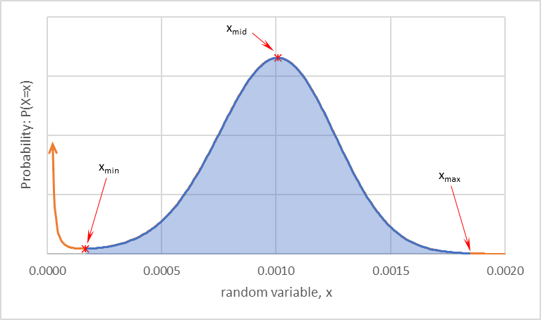
Fig. 11 The number-weighted normal distribution function approximated by dividing the volume-weighted distribution function by x³. The approximate mean and variance are computed by numerically integrating this function from x_min to x_max.

Sampling a normal distribution

MFIX-Exa samples the normal distribution with mean m_mean and standard deviation m_stddev to return an distribution observation.

amrex::Real observation;

do { observation = amrex::RandomNormal(m_mean, m_stddev, a_engine); }
while (!(m_min <= observation && observation <= m_max));

return observation;

The function amrex::RandomNormal returns one pseudo-random real number (double). The sample is discarded and the distribution is sampled again until the value satisfies \(\mathrm{xmin} \le x\) and \(x \le \mathrm{xmax}\).

log-normal distribution

The log-normal distribution is given by

\[f_X(x) = \frac{d}{dx}F_X(x) = \frac{1}{x \sigma \sqrt{2\pi}} \exp{\left(- \frac{(\mathrm{ln}(x) - \mu)^2 }{ 2 \sigma^2 }\right)}\]

where \(\mu\) and \(\sigma\) are parameters defining the distribution.

Note

\(\mu\) and \(\sigma\) are not the mean and standard deviation of \(x\). They are the mean and standard deviation of \(\mathrm{ln}(x)\). The mean (expectation), \(E(x)\), and variance, \(V(x)\), of the log-normal random variable are given by

\[E(x) = \exp{\left(\mu + \sigma^s/2\right)}\]

and

\[V(x) = \exp{\left(2\mu + 2\sigma^2\right)} - \exp{\left(2\mu + \sigma^2\right)}\]

respectively. See William Navidi [WN14] for an overview of log-normal distributions.

	Description	Type	Default
type	distribution weighting: number-weighted or volume-weighted	string	N/A
mean	mean of of the normal random variable, \(\mathrm{ln}(X)\)	Real	N/A
stddev	standard deviation of the normal random variable, \(\mathrm{ln}(X)\)	Real	N/A
min	Minimum particle diameter. Drawn samples below min are discarded and a new sample is drawn.	Real	N/A
max	Maximum particle diameter. Drawn samples above max are discarded and a new sample is drawn.	Real	N/A
bins	Number of bins used when discretizing the distribution to approximate the number of particles within an initial condition region.	int	64

In the following example, a cuboid with volume 0.001 m³ is filled with a volume-weighted log-normal distribution with the listed parameters. The minimum and maximum particle diameters are 0.23 mm and 3.00 mm, respectively.

Listing 12 Snippet of inputs defining a number-weighted log-normal distribution. This is not a complete input file.

# Regions for defining ICs and BCs
# -----------------------------------------------------------------------
mfix.regions = full-domain

regions.full-domain.lo  = 0.0  0.0  0.0
regions.full-domain.hi  = 0.1  0.1  0.1

# Initial Conditions
# -----------------------------------------------------------------------
ic.regions = full-domain

mfix.particle_init_type = Auto

# Full domain
#~~~~~~~~~~~~~~~~~~~~~~~~~~~~~~~~~~~~~~~~~~~~~~~~~~~~~~~~~~~~~~~~~>
ic.full-domain.fluid.volfrac  = 0.75

ic.full-domain.fluid.density  = 1.0
ic.full-domain.fluid.pressure = 0.0
ic.full-domain.fluid.velocity = 0.0  0.0  0.0

ic.full-domain.solids  = solid0

ic.full-domain.packing = random

ic.full-domain.solid0.volfrac   = 0.25
ic.full-domain.solid0.velocity  = 0.00  0.00  0.00

ic.full-domain.solid0.diameter = log-normal
ic.full-domain.solid0.diameter.type = volume-weighted
ic.full-domain.solid0.diameter.mean = -3.662955279
ic.full-domain.solid0.diameter.std  =  1.04
ic.full-domain.solid0.diameter.min  =   30.e-6  # (m)
ic.full-domain.solid0.diameter.max  = 3000.e-6  # (m)

ic.full-domain.solid0.density =  constant
ic.full-domain.solid0.density.constant  = 2500.0 # (kg/m^3)

An MFIX-Exa DEM simulation with these settings generates approximately 162,000 particles. The particle size distribution (open circles), and number-weighted (orange), and volume-weighted (blue) density functions are shown in Fig. 12.

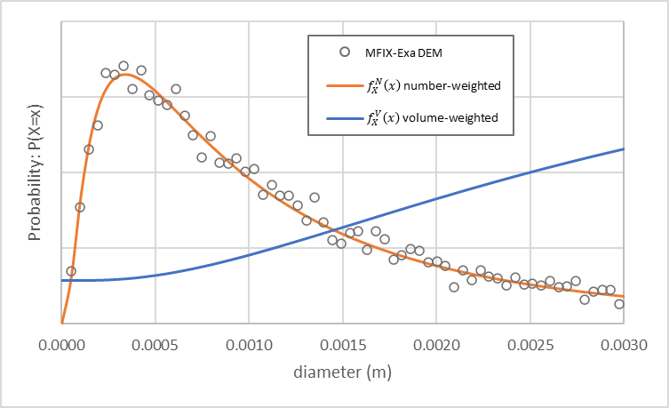
Fig. 12 MFIX-Exa DEM particle size distribution (open circles) and number-weighted (orange) and volume-weighted (blue) density functions.

An MFIX-Exa PIC simulation with the same settings generates approximately 410,000 parcels when pic.close_pack = 0.64, pic.parcels_per_cell_at_pack = 32, and the Eulerian mesh spacing \(\Delta x\) is 3.125 mm. Fig. 13 shows the parcel size distribution (open triangles) and number-weighted (orange) and volume-weighted (blue) density functions. Again, small closed circles indicate the effective particle distribution captured by the PIC parcels.

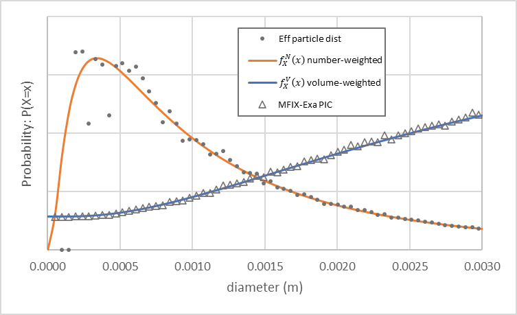
Fig. 13 MFIX-Exa PIC parcel size distribution (open triangles), number-weighted density function (orange), and volume-weighted density function (blue). Small closed circles indicated the particle size distribution modeled by the parcels.

Converting between number-weighted and volume-weighted parameters for log-normal distributions

As reported by El-Hilo [EH12], El-Hilo and Chantrell [EHC12], number-weighted and volume-weighted log-normal distributions use the same \(\sigma\) parameter

\[\sigma = \sigma_{N} = \sigma_{V}\]

while the parameter \(\mu\) is computed directly from the other distribution.

\[\begin{split}\begin{align} \mu_V =& \mu_N + 3.0\sigma^2 \\[10pt] \mu_N =& \mu_V - 3.0\sigma^2 \end{align}\end{split}\]

Sampling a log-normal distribution

Rather than sample the log-normal distribution, MFIX-Exa samples the normal distribution with mean m_mean and standard deviation m_stddev.

amrex::Real observation;

do { observation = amrex::RandomNormal(m_mean, m_stddev, a_engine); }
while (!(m_log_min <= observation && observation <= m_log_max));

return std::exp(observation);

The function amrex::RandomNormal returns one pseudo-random real number (double). The sample is discarded and the distribution is sampled again until the value satisfies \(\log \mathrm{xmin} \le \log x\) and \(\log x \le \log \mathrm{xmax}\). The log-normal variable is returned by applying the exponential function, \(x = \exp ( \log x )\).

uniform distribution

The uniform distribution is given by

(6)\[\begin{split}f_X(x) = \frac{d}{dx}F_X(x) = \begin{cases} \left(x_\mathrm{max} - x_\mathrm{min}\right)^{-1}, & \text{for} \; x \in \left[ x_\mathrm{min}, x_\mathrm{max} \right] \\ 0, & \text{otherwise} \end{cases}\end{split}\]

where \(x_\mathrm{min}\) and \(x_\mathrm{max}\) are the minimum and maximum particle diameters. The inputs used to specify the distribution are provided in the following table.

	Description	Type	Default
type	distribution weighting: number-weighted or volume-weighted	string	N/A
min	Minimum particle diameter. Drawn samples below min are discarded and a new sample is drawn.	Real	N/A
max	Maximum particle diameter. Drawn samples above max are discarded and a new sample is drawn.	Real	N/A
bins	Number of bins used when discretizing the distribution to approximate the number of particles within an initial condition region.	int	64

In the following example, a cuboid with volume 0.001 m³ is filled with a number-weighted uniform distribution. The minimum and maximum particle diameters are 0.25 mm and 1.75 mm, respectively.

Listing 13 Snippet of inputs defining a number-weighted uniform distribution. This is not a complete input file.

# Regions for defining ICs and BCs
# -----------------------------------------------------------------------
mfix.regions = full-domain

regions.full-domain.lo  = 0.0  0.0  0.0
regions.full-domain.hi  = 0.1  0.1  0.1

# Initial Conditions
# -----------------------------------------------------------------------
ic.regions = full-domain

mfix.particle_init_type = Auto

# Full domain
#~~~~~~~~~~~~~~~~~~~~~~~~~~~~~~~~~~~~~~~~~~~~~~~~~~~~~~~~~~~~~~~~~>
ic.full-domain.fluid.volfrac  = 0.95

ic.full-domain.fluid.density  = 1.0
ic.full-domain.fluid.pressure = 0.0
ic.full-domain.fluid.velocity = 0.0  0.0  0.0

ic.full-domain.solids  = solid0

ic.full-domain.packing = random

ic.full-domain.solid0.volfrac   = 0.05
ic.full-domain.solid0.velocity  = 0.00  0.00  0.00

ic.full-domain.solid0.diameter = uniform
ic.full-domain.solid0.diameter.type = number-weighted
ic.full-domain.solid0.diameter.min  =  250.e-6  # (m)
ic.full-domain.solid0.diameter.max  = 1750.e-6  # (m)

ic.full-domain.solid0.density =  constant
ic.full-domain.solid0.density.constant  = 2500.0 # (kg/m^3)

An MFIX-Exa DEM simulation with these settings generates approximately 110,000 particles. The particle size distribution (open circles), and number-weighted (orange), and volume-weighted (blue) density functions are shown in Fig. 14.

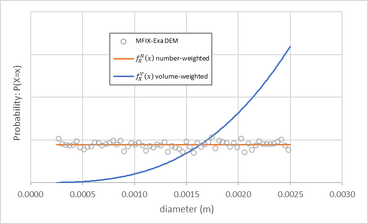
Fig. 14 MFIX-Exa DEM uniform particle size distribution (open circles) and number-weighted (orange) and volume-weighted (blue) uniform density functions.

An MFIX-Exa PIC simulation with the same settings generates approximately 410,000 parcels when pic.close_pack = 0.64, pic.parcels_per_cell_at_pack = 32, and the Eulerian mesh spacing \(\Delta x\) is 3.125 mm. Fig. 15 shows the parcel size distribution (open triangles) and number-weighted (orange) and volume-weighted (blue) density functions. Again, small closed circles indicate the effective particle distribution captured by the PIC parcels.

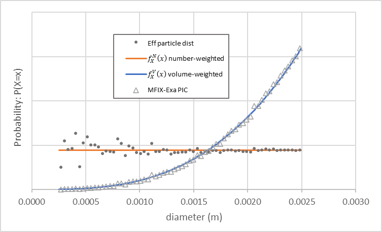
Fig. 15 MFIX-Exa PIC uniform parcel size distribution (open triangles), number-weighted (orange) and volume-weighted (blue) uniform density functions. Small closed circles indicated the particle size distribution modeled by the parcels.

Sampling a uniform distribution

DEM simulations where a number-weighted distribution is specified and PIC simulations where a volume-weighted distribution is specified compute a uniformly distributed variable \(rand \in \left( 0, 1 \right)\), then scale and translate the result such that \(x \in \left[ x_\mathrm{min}, x_\mathrm{max} \right)\).

amrex::Real rand = amrex::Random(a_engine);

return m_min + (m_max-m_min)*rand;

The function amrex::Random returns one pseudo-random real number (double) from a uniform distribution between 0.0 and 1.0 (0.0 included, 1.0 excluded).

Inverse sampling is used when a volume-weighted distribution is specified for a DEM simulation and when a number-weighted distribution is specified for a PIC simulation. This approach generates random variates from the continuous distribution function \(F\) using the inverse function \(F^{-1}\).

If \(\mathcal{U}\) is a uniform random variable on the interval \([0,1]\) and \(F\) is a continuous cumulative distribution function on \([a,b]\) with inverse

\[F^{-1}(u) = \inf \left\{ x: F(x) = u \right\}\]

then \(F^{-1}(\mathcal{U})\) has cumulative distribution function \(F\) (adapted from Devroye [Dev86]).

The number-weighted density function, \(f_X^N(x)\), is computed from a specified volume-weighted density function by dividing (6) by \(x^3\). The brace notation indicating that the density function is zero for \(x \notin \left[ x_\mathrm{min}, x_\mathrm{max} \right]\) is dropped for conciseness.

\[f_X^N(x) = \frac{1}{x^3 (x_{\mathrm{min}} - x_{\mathrm{max}})}\]

The cumulative distribution function and its inverse are

\[\mathrm{Pr}\left(X \le x\right) = F_X^N(x) = \frac{ \int_{a}^{x} f_X^N(y) dy }{\int_{a}^{b} f_X^N(y) dy } = \frac{ b^2(x^2-a^2)}{x^2(b^2 - a^2)}\]

and

\[{F_X^N}^{-1}(u) = \frac{ab}{\sqrt{b^2 - u(b^2 -a^2)}}\]

where \(a = x_{\mathrm{min}}\) and \(b = x_{\mathrm{max}}\). To sample \(f_X^V(x)\), a uniformly distributed variable \(u \in \mathcal{U}(0,1)\) is generated and substituted into the inverse cumulative distribution function.

amrex::Real rand = amrex::Random(a_engine);

amrex::Real const b(m_max);
amrex::Real const a(m_min);

amrex::Real const a2(a*a), b2(b*b);

return (a*b)/std::sqrt(b2 - rand*(b2-a2));

Similarly, a volume-weighted density function, \(f_X^V(x)\), is computed from a number-weighted distribution by multiplying (6) by \(x^3\). Again, the brace notation indicating that the density function is zero for \(x \notin \left[ x_\mathrm{min}, x_\mathrm{max} \right]\) is dropped for conciseness.

\[f_X^V(x) = \frac{x^3}{(x_{\mathrm{min}} - x_{\mathrm{max}})}\]

The cumulative distribution function and its inverse are

\[\mathrm{Pr}\left(X \le x\right) = F_X^V(x) = \frac{ \int_{a}^{x} f_X^V(y) dy }{\int_{a}^{b} f_X^V(y) dy } = \frac{ x^4 - a^4 }{ b^4 - a^4 }\]

and

\[{F_X^V}^{-1}(u) = \left(a^4 + u(b^4 - a^4)\right)^{1/4}\]

where \(a = x_{\mathrm{min}}\) and \(b = x_{\mathrm{max}}\). To sample \(f_X^V(x)\), a uniformly distributed variable \(u \in \mathcal{U}(0,1)\) is generated and substituted into the inverse cumulative distribution function.

amrex::Real rand = amrex::Random(a_engine);

amrex::Real const b(m_max);
amrex::Real const a(m_min);

amrex::Real const a4(a*a*a*a), b4(b*b*b*b);

return std::pow(a4 + rand*(b4-a4),0.25);

custom distribution

A user-defined custom distribution can be specified by providing discrete probabilities via a text file.

	Description	Type	Default
custom	File name of user-defined distribution	string	N/A
min	Minimum particle diameter. Drawn samples below min are discarded and a new sample is drawn.	Real	N/A
max	Maximum particle diameter. Drawn samples above max are discarded and a new sample is drawn.	Real	N/A
interpolate	Enable linear interpolation between discrete bins. This option is only available when the initial distribution probability is zero.	bool	false

The distribution input file contains four components:

• line 1: number of distribution entries (integer)

• line 2: specifies the distribution as CDF or PDF (string)

• line 3: comment or blank line (unused by solver)

• remaining lines define the bin and probability (Real Real)

The following sections provide a few examples of custom distribution configurations.

Bidisperse mixutre without interpoaltion

In the following example, a cuboid with volume 0.001 m³ is filled with a number-weighted distribution. The distribution is a 50/50 mixture of two particle sizes.

Listing 14 Snippet of inputs defining a number-weighted custom distribution. This is not a complete input file.

# Regions for defining ICs and BCs
# -----------------------------------------------------------------------
mfix.regions = full-domain

regions.full-domain.lo  = 0.0  0.0  0.0
regions.full-domain.hi  = 0.1  0.1  0.1

# Initial Conditions
# -----------------------------------------------------------------------
ic.regions = full-domain

mfix.particle_init_type = Auto

# Full domain
#~~~~~~~~~~~~~~~~~~~~~~~~~~~~~~~~~~~~~~~~~~~~~~~~~~~~~~~~~~~~~~~~~>
ic.full-domain.fluid.volfrac  = 0.95

ic.full-domain.fluid.density  = 1.0
ic.full-domain.fluid.pressure = 0.0
ic.full-domain.fluid.velocity = 0.0  0.0  0.0

ic.full-domain.solids  = solid0

ic.full-domain.packing = random

ic.full-domain.solid0.volfrac   = 0.05
ic.full-domain.solid0.velocity  = 0.00  0.00  0.00

ic.full-domain.solid0.diameter = custom
ic.full-domain.solid0.diameter.custom = bidisperse-pdf.dist
ic.full-domain.solid0.diameter.type = number-weighted

ic.full-domain.solid0.density =  constant
ic.full-domain.solid0.density.constant  =  2500.0    # (kg/m^3)

ic.full-domain.solid0.density =  constant
ic.full-domain.solid0.density.constant  = 2500.0 # (kg/m^3)

Listing 15 Custom distribution defining a 50/50 mixture of two particle sizes.

2
PDF
# bidisperse mixture
 500.e-6  0.5
1000.e-6  0.5

An MFIX-Exa DEM simulation with these settings generates approximately 180,000 particles with half of the particles having diameter 0.5 mm and half have diameter 1.0 mm. An MFIX-Exa PIC simulation with the same settings generates approximately 82,000 parcels when pic.close_pack = 0.64, pic.parcels_per_cell_at_pack = 32, and the Eulerian mesh spacing \(\Delta x\) is 3.125 mm. Approximately 10% of the parcels have diameter 0.5 mm and 90% have diameter 1.0 mm.

Bimodal mixutre

The following example uses the same layout as the previous example, however the custom distribution is of a CDF describing a bimodal distribution created by combining two normal distributions.

ic.full-domain.solid0.volfrac   = 0.05
ic.full-domain.solid0.velocity  = 0.00  0.00  0.00

ic.full-domain.solid0.diameter = custom
ic.full-domain.solid0.diameter.custom = bimodal-cdf.dist
ic.full-domain.solid0.diameter.type = number-weighted

Listing 16 Custom bimodal distribution created by combining two normal distributions

25
CDF
# bimodal distribution created from two normal distributions
0.000144  0.0000
0.000240  0.0063
0.000336  0.0360
0.000384  0.0818
0.000416  0.1356
0.000432  0.1919
0.000456  0.2495
0.000480  0.3053
0.000496  0.3587
0.000528  0.4055
0.000568  0.4447
0.000584  0.4822
0.000600  0.5191
0.000616  0.5566
0.000632  0.5958
0.000664  0.6408
0.000704  0.6942
0.000720  0.7501
0.000752  0.8075
0.000768  0.8638
0.000784  0.9177
0.000816  0.9635
0.000864  0.9932
0.000960  0.9995
0.001056  1.0000

An MFIX-Exa DEM simulation with these settings generates approximately 2,285,000 particles. The particle size distribution (open circles), and number-weighted (orange), and volume-weighted (blue) density functions are shown in Fig. 16.

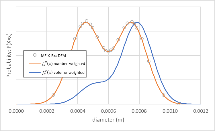
Fig. 16 MFIX-Exa DEM custom bimodal particle size distribution (open circles) and number-weighted (orange) and volume-weighted (blue) density functions.

An MFIX-Exa PIC simulation with the same settings generates approximately 82,000 parcels when pic.close_pack = 0.64, pic.parcels_per_cell_at_pack = 32, and the Eulerian mesh spacing \(\Delta x\) is 3.125 mm. The parcel size distribution shown in Fig. 17 (open triangles) follows the volume-weighted density function. Small closed circles illustrate the effective particle size distribution, computed by multiplying each observation by the parcel statistical weight.

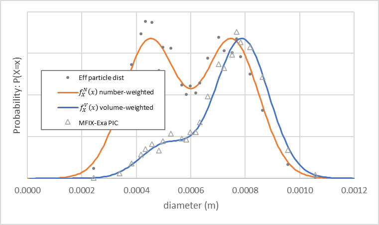
Fig. 17 MFIX-Exa PIC custom bimodal parcel size distribution (open triangles), number-weighted (orange) and volume-weighted (blue) density functions. Small closed circles indicated the particle size distribution modeled by the parcels.

Measured size distribution

The final example uses the same layout as the previous examples, however the custom distribution is a CDF describing an experimentally measured size distribution and the distribution type is volume-weighted.

ic.full-domain.solid0.volfrac   = 0.05
ic.full-domain.solid0.velocity  = 0.00  0.00  0.00

ic.full-domain.solid0.diameter = custom
ic.full-domain.solid0.diameter.custom = qicpic-cdf.dist
ic.full-domain.solid0.diameter.type = volume-weighted

Listing 17 Measured custom distribution

32
CDF

0.00025   0.0013499
0.000298387   0.00250452
0.000346774   0.00448884
0.000395161   0.00777403
0.000443548   0.0130136
0.000491935   0.0210638
0.000540323   0.0329789
0.00058871   0.0499683
0.000637097   0.0733046
0.000685484   0.104184
0.000733871   0.143547
0.000782258   0.191886
0.000830645   0.24907
0.000879032   0.314239
0.000927419   0.385785
0.000975806   0.461453
0.00102419   0.538547
0.00107258   0.614215
0.00112097   0.685761
0.00116935   0.75093
0.00121774   0.808114
0.00126613   0.856453
0.00131452   0.895816
0.0013629   0.926695
0.00141129   0.950032
0.00145968   0.967021
0.00150806   0.978936
0.00155645   0.986986
0.00160484   0.992226
0.00165323   0.995511
0.00170161   0.997495
0.00175   0.99865

An MFIX-Exa DEM simulation with these settings generates approximately 963,000 particles. The particle size distribution (open circles), and number-weighted (orange plus), and volume-weighted (blue cross) probabilities are shown in Fig. 18.

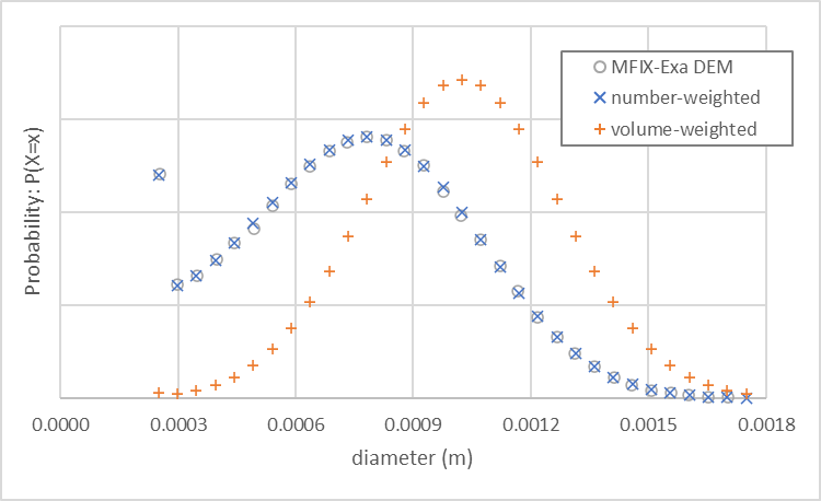
Fig. 18 MFIX-Exa DEM custom bimodal particle size distribution (open circles) and number-weighted (orange plus) and volume-weighted (blue cross ) probabilities.

An MFIX-Exa PIC simulation with the same settings generates approximately 164,000 parcels when pic.close_pack = 0.64, pic.parcels_per_cell_at_pack = 64, and the Eulerian mesh spacing \(\Delta x\) is 3.125 mm. The parcel size distribution shown in Fig. 19 (open triangles) follows the volume-weighted probabilities. Small closed circles illustrate the effective particle size distribution, computed by multiplying each observation by the parcel statistical weight.

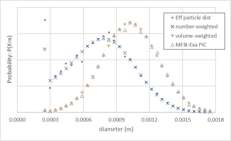
Fig. 19 MFIX-Exa PIC custom bimodal parcel size distribution (open triangles), number-weighted (orange plus) and volume-weighted (blue cross) probabilities. Small closed circles indicated the particle size distribution modeled by the parcels.