DOE Methods
The sampling methods implemented in the Design of Experiments node do not call external python libraries and are directly coded within Nodeworks. Therefore, a brief overview of the different hard-coded methods are provided here.
All these methods return an array of samples between 0 and 1. These samples are then converted to the appropriate ranges as specified.
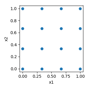
Factorial
Factorial constructs a full factorial design for an arbitrary number of factors at an arbitrary number of levels. This typically results in the largest number of samples since every possible combination of factors is produced.
The code here was inspired by pyDOE: Factorial
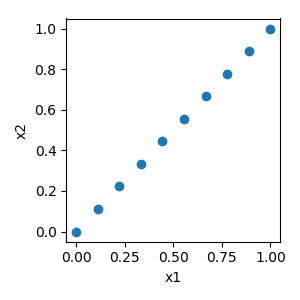
Covary
Covary simply varies one or more factors linearly together with a slope of 1 and an intercept of 0, i.e. \(y=x\).
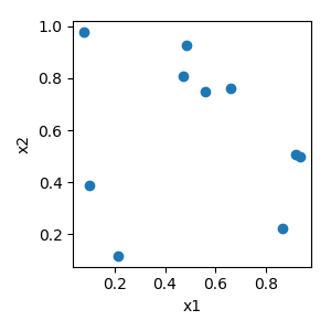
Monte Carlo
Numpy’s random.uniform method is used to create the random samples. If a seed is used to fix the internal random generator, then random.seed is called before calling random.uniform.
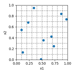
Latin Hypercube
The sample space is first divided into equal intervals. In each interval, random points are selected using Numpy’s, random.rand. Finally, points are randomly paired to make samples using Numpy’s random.permutation.
Similarly to the Monte Carlo, if a seed is used to fix the internal random generator, then random.seed is called before entering the routine. This allows for reproducible designs.
The code here was inspired by pyDOE: LHS
Generally, the basic Latin Hypercube algorithm does a better job of spacing filling than Monte Carlo. However, there are techniques to improve the spacing filling of the basic Latin Hypercube. Three are implemented here.
maximin
If maximin is selected, then a user defined number (iterations) of basic
Latin Hypercubes are constructed. The minimum distance between any two points is
determined for each design using Scipy’s pairwise distance
function. The design with the maximum minimum distance is returned.
ratio
Similar to maximin, ratio constructs a user defined number
(iterations) of basic Latin Hypercubes. A ratio of the maximum distance
between any two points over the minimum distance between any two points
(\(max(dist)/min(dist)\)) is calculated using
Scipy’s pairwise distance
function for each design. The design with the minimum ration is returned.
genetic
The genetic option follows the methodology described by Jin et al.
[Jin2005] for taking a design and using an enhanced stochastic evolutionary
(ESE) algorithm to optimize the design by columnwise operations, called
element-exchange, which interchanges two distinct elements in a column. This
technique allows for variables in samples to be exchanged to improve the
space filling of the original design without changing the original variables.
This guarantees that the resulting “optimized” design will still be a latin
hypercube.
The number of exchanges (\(J\)), inner iterations (\(M\)), as well as
the warming and cooling parameters are all calculated based on the
recommendations made by Jin et al. [Jin2005]. The number of outer iterations
is user selected (iterations). The objective function is the Wrap-Around
L2-Discrepancy from Eq.5 of [Fang2001].
The actual python implementation of the L2-Discrepancy was extracted from damar-wicaksono/gsa-module (MIT license).
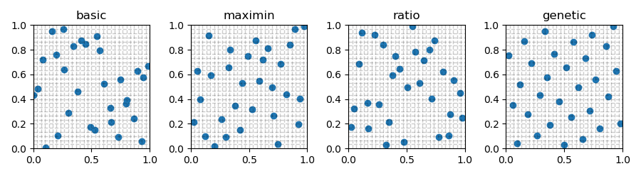
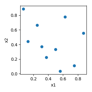
Latin Hypercube techniques with 2 variables, 30 samples, and 1000 iterations
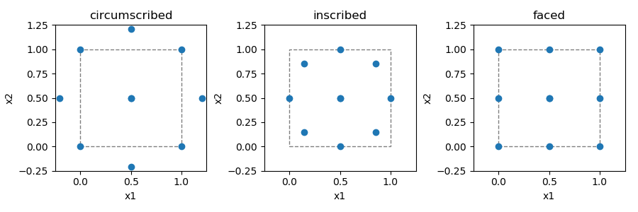
Central Composite
Central composite design is a combination of a 2-level full-factorial and a star. There are three different options for the relation between the star points and the corner points:
- circumscribed - star points are at some distance
alphafrom the center. - inscribed - uses the factors settings as the star points and creates a factorial or fractional factorial design within those limits.
- faced - the star points are at the center of each face of the factorial space.
alpha can be:
| orthogonal | \(\sqrt{n_{variables}{{1+ 1/n_{axial}}\over{1+1/k_{factorial}}}}\) |
| rotatable | \(\sqrt[4]{k_{factorial}}\) |
The code here was inspired by pyDOE: Composite
Sobol
The sobol implementation was adapted from jburkardt and can handle a maximum of 40 variables.
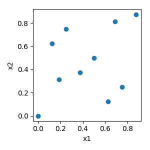
Hammersly
The Hammersly method is a sampling technique based on the low discrepancy Hammersly sequence. It provides more uniform samples as compared to Monte Carlo.
The code here was adapted from PhaethonPrime which is based on Sampling with Hammersley and Halton Points
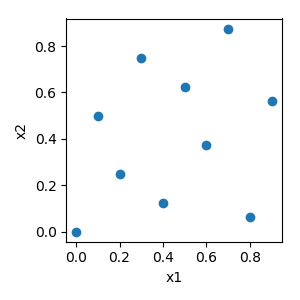
Halton
Similar to the Hammersly method, the Halton method is a sampling technique based on the low discrepancy Halton sequence. It provides more uniform samples as compared to Monte Carlo.
The code here was adapted from PhaethonPrime which is based on Sampling with Hammersley and Halton Points
References
| [Fang2001] | K.T. Fang and C.X. Ma, “Wrap-Around L2-Discrepancy of Random Sampling, Latin Hypercube, and Uniform Designs,” Journal of Complexity, vol. 17, pp. 608-624, 2001. |
| [Jin2005] | (1, 2) Ruichen Jin, Wei Chen, Agus Sudjianto, “An efficient algorithm for constructing optimal design of computer experiments”, Journal of Statistical Planning and Inference, vol. 134, pp. 268-287, 2005, ISSN 0378-3758, https://doi.org/10.1016/j.jspi.2004.02.014. |