Ex. 5: Deterministic Calibration¶

Suppose we have a complex model with numerous unknown parameters that we want to calibrate to experimental data (well not that complex):

\[f(x, y) = |x|^a + |y|^b\]

Where the model inputs are \(x\) and \(y\), and \(a\) and \(b\) are unknown model parameters. We can use nodes available in nodeworks to explore a collection of \(a\) and \(b\) parameter values and fit a surrogate model to the response. We can then evaluate the surrogate model at experimental conditions and compare the response of the surrogate model to the experimental response. Finally, we can calibrate the \(a\) and \(b\) parameters to the experimental data using the optimization node.

Step 1: Sample the model¶

We need to generate samples for all four variables. To do this, add a Design of Experiments node. Add the four variables and adjust the ranges to match the following:

Variable	From	To
x	-1.0	1.0
y	-1.0	1.0
a	1.0	4.0
b	1.0	4.0

Next, go to the Design tab of the Design of Experiments node. Change the Method to latin hypercube and the samples to 100. Finally, press Build to generate the samples.

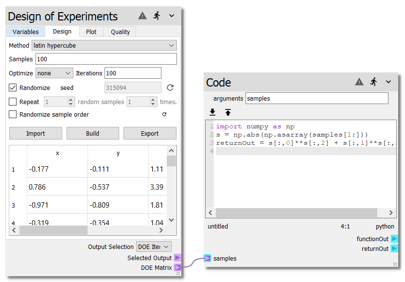
Add a Code node next to the Design of Experiments node. Create a new terminal by entering “samples” in the arguments field. Copy and paste the following python code into the editor. This code will evaluate the model for each sample.

import numpy as np
s = np.abs(np.asarray(samples[1:]))
returnOut = s[:,0]**s[:,2] + s[:,1]**s[:,3]

Finally, connect the DOE Matrix terminal of the Design of Experiments node to the samples terminal of the Code node. Your sheet should now look like the following:

Step 2: Build the surrogate¶

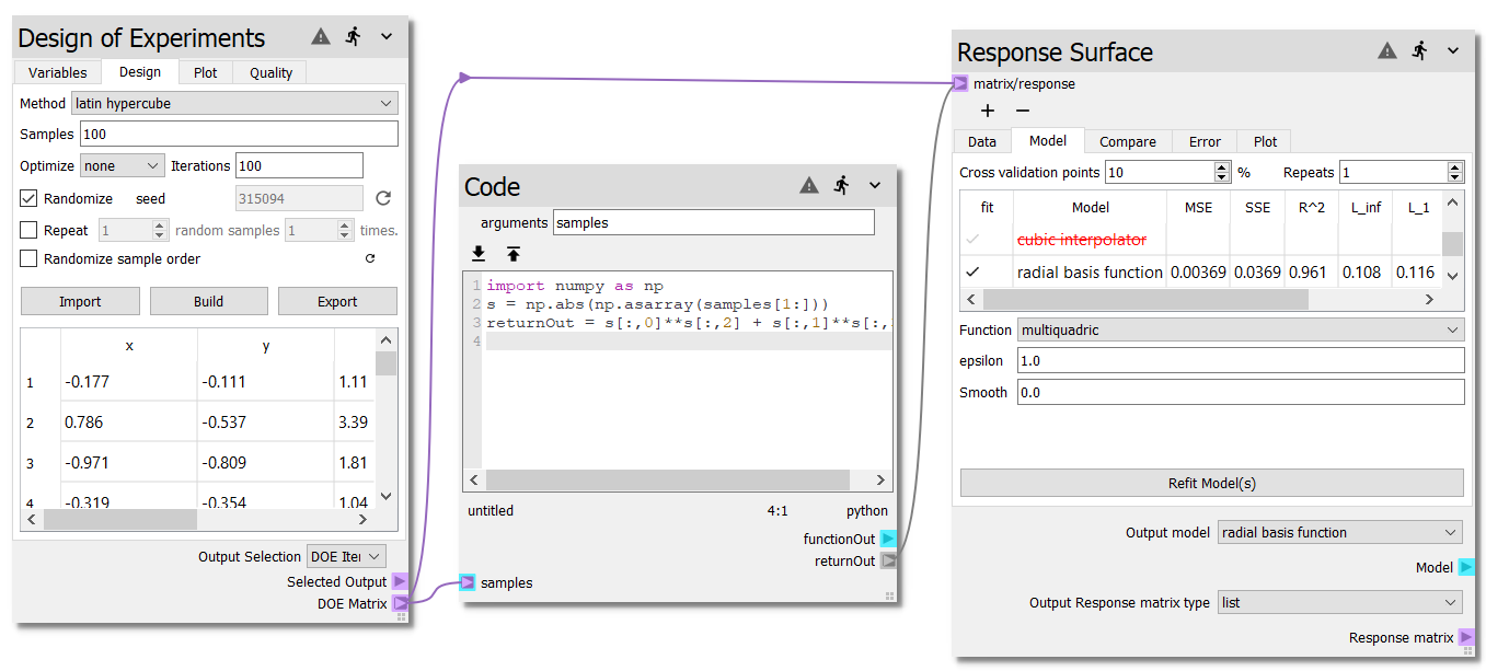
Now we will construct a surrogate model to represent the response of the model. Add a Response Surface node next to the Code node. Connect the returnOut terminal from the Code node to the matrix/response terminal on the Response Surface node. Next, connect the DOE Matrix terminal of the Design of Experiments node to the matrix/response terminal on the Response Surface node.

On the Model tab of the Response Surface node, check the check mark next to the radial basis function model. Run the sheet by pressing the play button. The sheet should now look like:

Step 3: Generate experimental data¶

For this particular example, we are going to generate experimental data. This allows use to play with the experimental data and explore the effects of samples and noise on the effectiveness of the calibration. You can also read data from *.csv files.

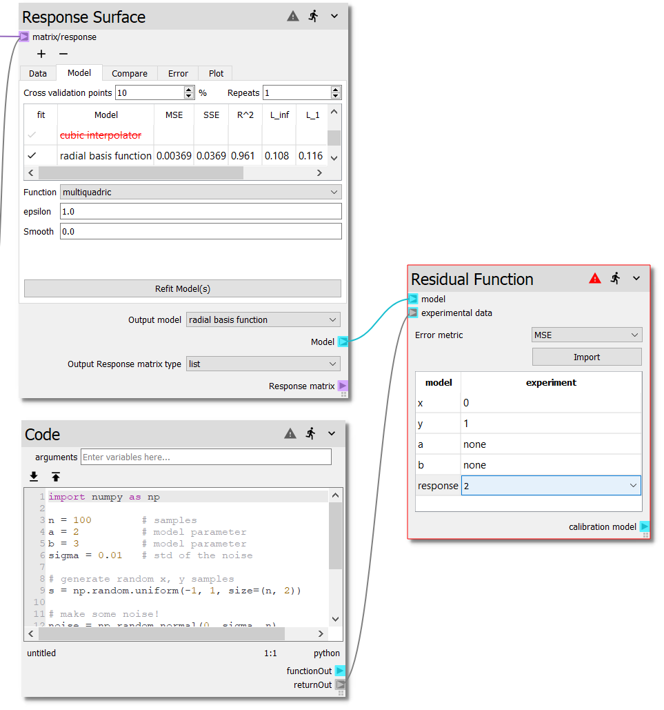
Add another Code node below the Response Surface node. Copy and paste the following python code into the editor.

import numpy as np

n = 100        # samples
a = 2          # model parameter
b = 3          # model parameter
sigma = 0.01   # std of the noise

# generate random x, y samples
s = np.random.uniform(-1, 1, size=(n, 2))

# make some noise!
noise = np.random.normal(0, sigma, n)

# calculate the response
r = np.abs(s[:,0])**a + np.abs(s[:,1])**b + noise

# combine the samples (x, y) with the response (r)
returnOut = np.hstack((s, np.atleast_2d(r).T))

Step 4: Calibrate¶

We are now ready to compare the model with the experimental data and minimize the error. Add a Residual Function node next to the Response Surface node. Connect the Model terminal of the Response Surface node to the model terminal of the Residual Function node. Also, connect the returnOut from the second Code node to the experimental data terminal of the Residual Function node.

Press play to run the sheet and populate the table of the Residual Function node. Now that the table is populated, we can map the experimental values to the model inputs. You will see the red error indication around Residual Function node with Show Error message icon on the top right of the node, which is normal as the Experimental dataset is not mapped to the surrogate model parameters.

To map the experimental values to the model parameters, Double-click the cell on the x row, experiment column and select 0 from the combo-box. This will map the first column of the experimental data to the \(x\) value of the model. Likewise, select 1 for the y row and 2 for the response row. Your sheet should now look like the following.

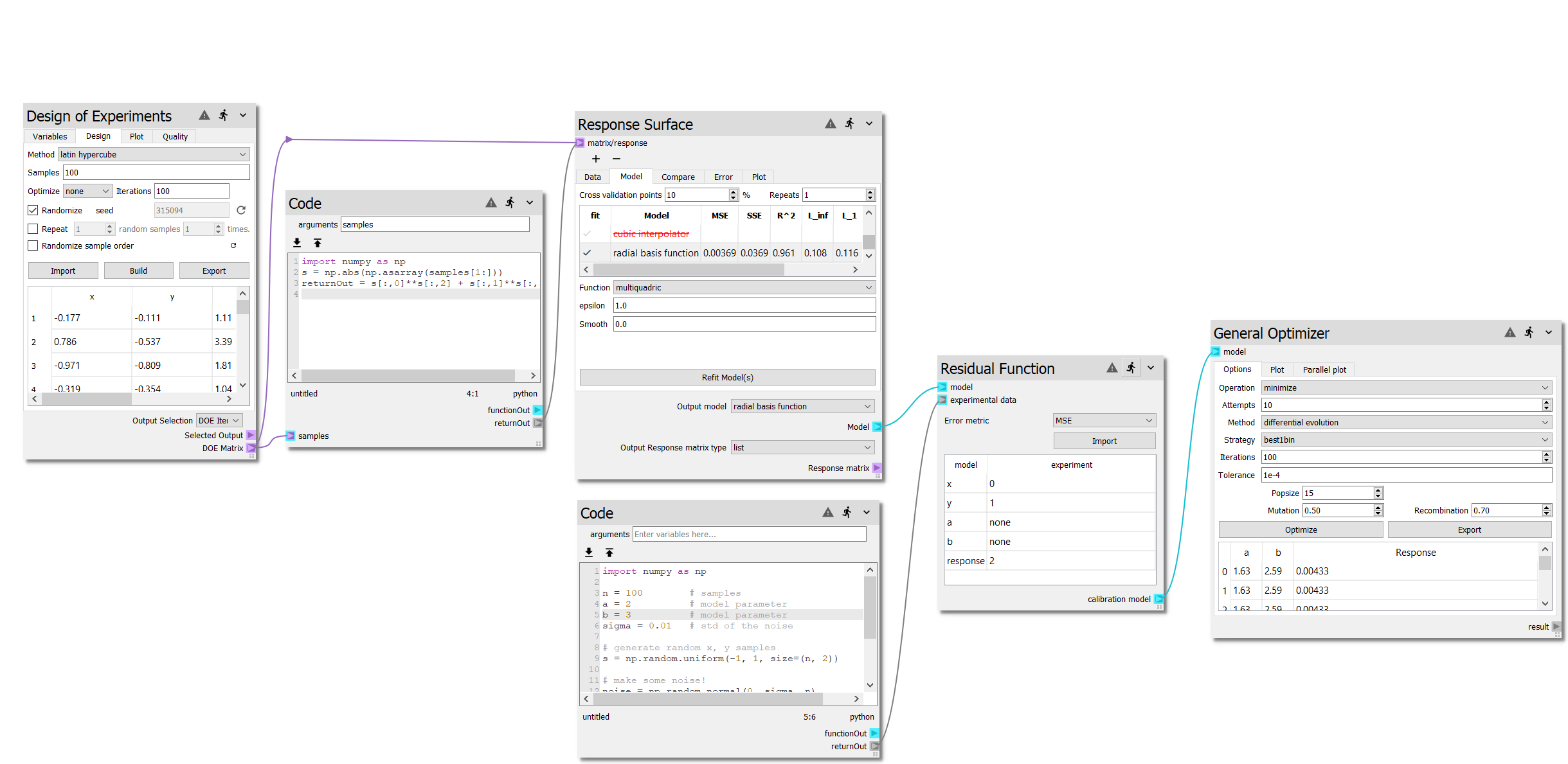
Finally, add a General Optimizer node next to the Residual Function node. Connect the calibration model terminal of the Residual Function node to model terminal of the General Optimizer node. On the General Optimizer node, change the number of attempts to 10. Finally, press play to run the sheet. The complete sheet should look like the following, note that the Latin Hypercube samples in Response Surface node and optimization results shown in General Optimizer might be different form your worksheet due to random sample generation:

Step 5: How close did it get?¶

In the second code node, we specified \(a = 2\) and \(b = 3\) when generating the experimental data. The General Optimizer node minimized the error between the model and the experiment data. In this particular instance, out of the 10 optimization attempts, the minimum error resulted in \(a = 1.63\) and \(b = 2.59\). So why are these not exactly \(a = 2\) and \(b = 3\)?

Well, there are random processes involved in generating the samples and noise added to the experimental data. Play with the number of model samples (Design of Experiments node), using other surogate models (Response Surface node), and the amount of samples and noise in the experimental data (n and sigma in the second Code node). How close can you get?

For example, changing the number of samples of the model from 100 to 500 in the Design of Experiments node and re-running the sheet resulted in a more accurate response surface. The General Optimizer then found the optimal values to be \(a = 1.97\) and \(b = 3.18\).