1. Eulerian01: athermal, constant density

1.1. Description

Consider a system with a fluid comprised of two chemical species, \(A\) and \(B\), with the transfer of species given by the reversible homogeneous reaction,

(1.1)\[A(g) \leftrightarrow B(g)\]

If both species have the same molecular weight, specific heat, and enthalpy of formation, then the mixture molecular weight, system temperature, and density are constant. The evolution of species mass in the absence of convection and diffusion is given by

(1.2)\[\rho\frac{\partial X_{A}}{\partial t} = \dot{\omega}_{A}\]

where \(\rho\) is density; \(X_A\) is the mass fraction of species \(A\); and \(\dot{\omega}_{A}\) is the net rate of production (consumption if negative) of species \(A\).

A manufactured solution for species \(A\) is

(1.3)\[X_A(t) = X_A^0 - \sin(6\pi t)/4\]

where \(X_A^0 = X_A(t=0)\) is the initial mass fraction of species \(A\). Taking the derivative with respect to time, and substituting the result into Eq.1.2 gives

(1.4)\[\dot{\omega}_A = -\rho 3\pi \cos(6\pi t)/2\]

which has units of kg·m\(^{-3}\)· sec\(^{-1}\). Two modifications are required to implement this Eulerian reaction rate into MFIX-Exa:

• Eq. Eq.1.4 needs to be divided by the molecular weight of species A because Eulerian reaction rates in MFIX-Exa are provided in units of mol·m\(^{-3}\)· sec\(^{-1}\).

• The negative sign is omitted because species \(A\) is a reactant. Specifically, by inspection of chemical equation Eq.1.1, species \(A\) is a reactant when the rate is positive (forward reaction), and a product when the rate is negative (backward reaction).

The resulting Eulerian reaction rate is

(1.5)\[R_A = \frac{\rho 3\pi \cos(6\pi t)}{2 M_A}\]

1.2. Setup

The domain is a single cuboid cell with 0.0025 m edge length and convection and diffusion terms are set to zero for all governing equations. The fluid has a constant temperature of 300 K at 60,795 Pa, and the initial composition is \(X_A=X_B=0.5\). The density is chosen to be 2 kg·m\(^{-3}\); therefore, the component and mixture molecular weights are computed from the ideal gas law \(M=\rho RT / p_{therm} \approx 0.0821\) kg·mol\(^{-1}\).

1.3. Results

The test is run at five fixed time-step sizes with a refinement factor of 2: 0.2, 0.1, 0.05, 0.025, 0.0125 milliseconds. The \(L_1\)-norm is computed by dividing the sum of the absolute difference between the analytical and numerical solution over all time steps by the total number of time steps.

\[L_1 = \frac{\sum_n \| X_A(t_n) - X_A^{\mathrm{\texttt{MFIX-Exa}}}\|}{n}\]

1.3.1. Forward Euler

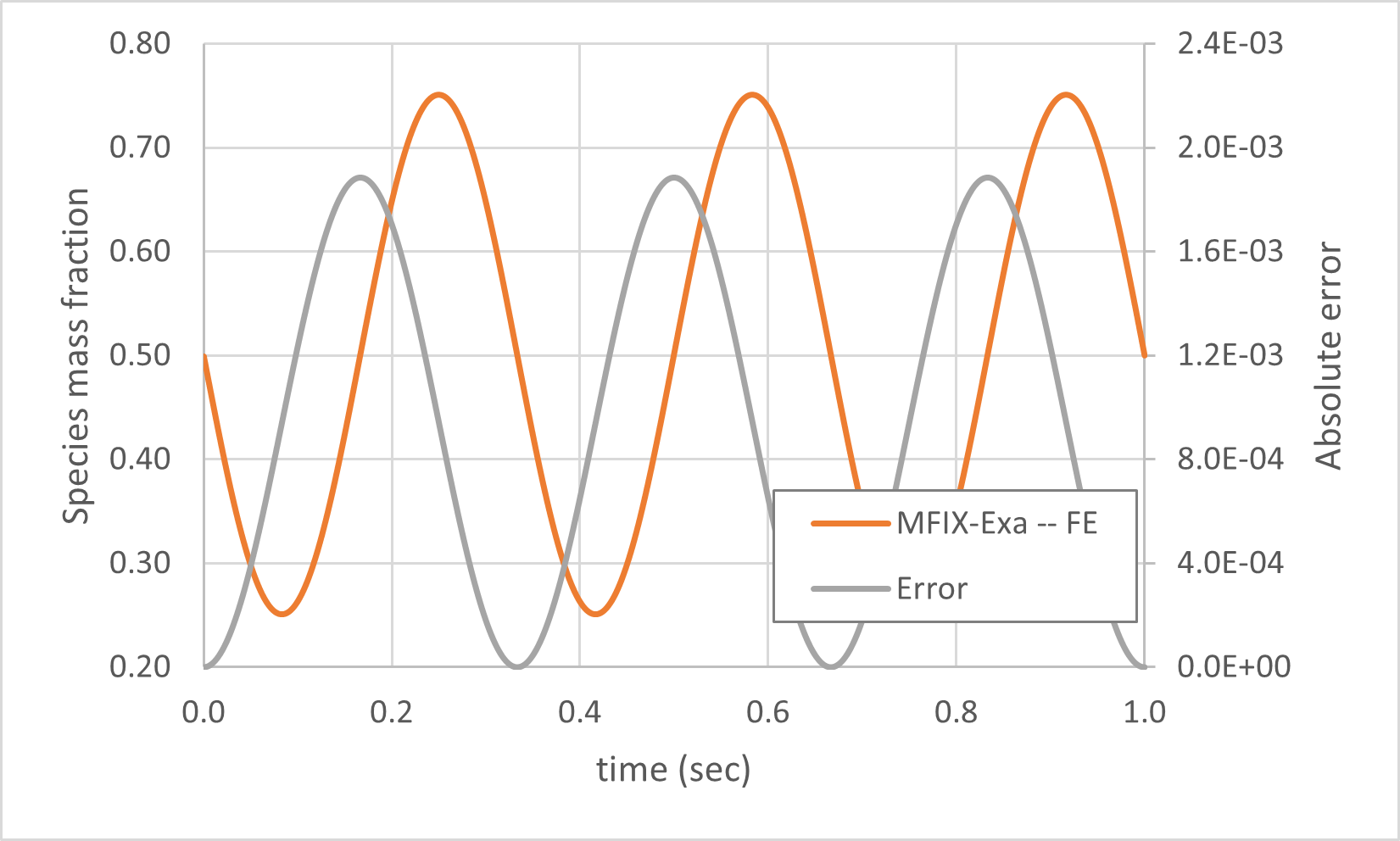
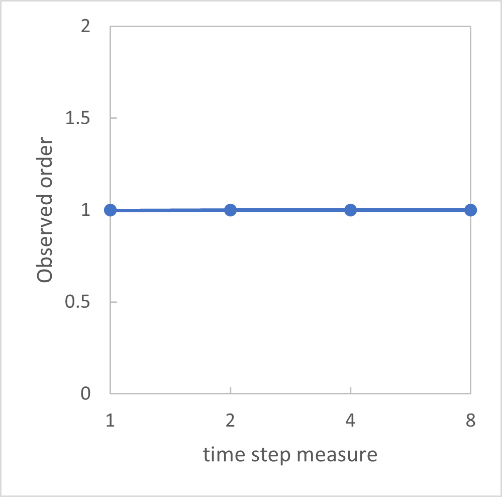
The analytical solution and absolute error with dt = 0.2 msec are shown in Fig. 1.1. The \(L_1\) norm is used to compute the observed order of accuracy shown in Fig. 1.2.

Fig. 1.1 Numerical solution for species mass fraction and absolute error.

Fig. 1.2 Observed order of species mass fraction.