3.6. Three Dimensional DEM Hopper
This tutorial shows how to create a three dimensional granular flow DEM simulation. The model setup is:
Property |
Value |
|---|---|
geometry |
5 cm diameter hopper |
mesh |
10 x 25 x 10 |
solid diameter |
0.003 m |
solid density |
2500 kg/m2 |
gas velocity |
NA |
temperature |
298 K |
pressure |
NA |
3.6.1. Create a new project
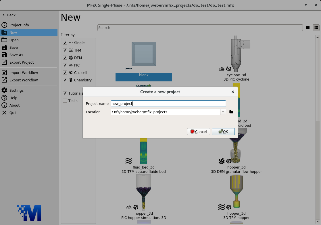
On the main menu, select
New projectCreate a new project by double-clicking on “Blank” template.
Enter a project name and browse to a location for the new project.
When prompted to enable SMS workflow, answer No, we will use the standard workflow for this tutorial.
3.6.2. Select model parameters
On the
Modelpane, enter a descriptive text in theDescriptionfieldSelect “Discrete Element Model (MFiX-DEM)” in the
Solverdrop-down menuCheck the
Disable Fluid Solver (Pure Granular Flow)check-box.

3.6.3. Enter the geometry
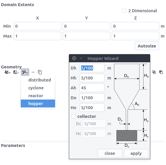
On the Geometry pane:
Select the
 wizard menu and select the
 hopperwizardSelect
applyto build the hopper stl filePress the
Autosizebutton to fit the domain extents to the geometryPress the
 Reset View icon on the top-left corner of the Model window
3.6.4. Enter the mesh
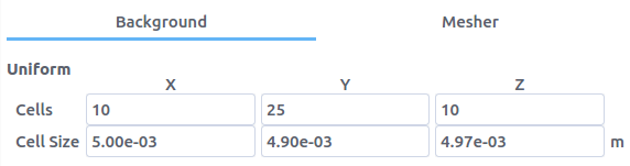
On the Mesh pane, Background sub-pane:
Enter
10for the x cell valueEnter
25for the y cell valueEnter
10for the z cell value
On the Mesh pane, Mesher sub-pane:
Enter
0.0in theFacet Angle Tolerance
3.6.5. Create regions for initial and boundary condition specification
Select the Regions pane. By default, a region that covers the
entire domain is already defined.
A region for the hopper walls (STL) is needed to apply a wall boundary condition to:
click the
 button to create a region that encompasses the entire
domain
button to create a region that encompasses the entire
domainchange the name of the region to a descriptive
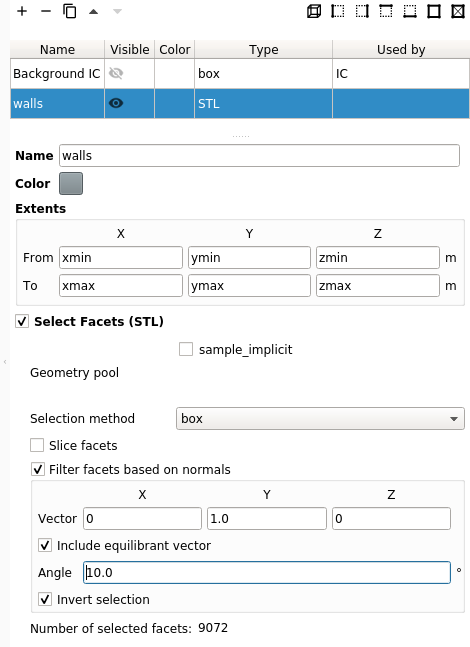
namesuch as “walls”Check the
Select Facets (STL)check-box to turn the region into a STL region. The facets of the hopper should now be selected.
In order to allow the particles to leave the domain through the bottom, the facets at the bottom of the hopper need to be deselected. There are three ways to accomplish this:
Change the
Y Mindomain extent value on the geometry pane by a small amount so that those facets fall outside the simulation domain (for example, change the value to-0.0974).Change the
Y Fromregion extent value on the regions pane for this STL region by a small amount so that those facets fall outside the region (for example, change the value toymin+0.0001)Or, use the
Filter facets based on normalsoption on the region pane.
For this example, use option 3 to filter the facets that have normals pointed in
the Y direction by:
Select
boxfrom theSelection methoddrop-down.Uncheck
Slice facets.Check the
Filter facets based on normalscheck-boxEnter a vector pointed in the positive
Ydirection by entering0,1, and0in the x, y, z fields, respectivelyCheck the
Include equilibrant vectorto include facets with normals in the opposite direction of the vector (-x, -y, -z)Enter an angle of
10in theanglefield to include facets with normals within 10 degrees of the filter vectorCheck the
Invert Selectioncheck box to de-select facets that fall along the filter vector and select all the other facets
All the facets, except for the facets at the top and bottom, of the hopper should now be selected.
Create a region to apply a pressure outlet boundary condition to allow particles to leave the domain:
Click the

Enter a name for the region in the
Namefield (“outlet”)
Finally, create a region to initialize the solids:
Click the
Enter a name for the region in the
Namefield (“solids”)Enter
ymin/3in theFrom YfieldEnter
0in theTo Yfield
3.6.6. Create a solid
On the Solids pane
Click the
 button to create a new solid
Enter a descriptive name in the
Namefield (“solids”)Keep the model as “Discrete Element Model (MFiX-DEM)”)
Enter the particle diameter of
0.003m in theDiameterfieldEnter the particle density of
2500kg/m2 in theDensityfield
In the DEM sub-pane, check Enable automatic particle generation check-box
3.6.7. Create Initial Conditions
On the Initial conditions pane
Click the
button to create a new initial conditionOn the
Select Regiondialog, select the “solids” region and clickOKOn the
solidssub-pane, enter0.4in theVolume fractionfield
3.6.8. Create Boundary Conditions
Select the Boundary conditions pane and create a wall boundary condition for
the hopper by:
clicking the
buttonOn the
Select Regiondialog, select “No Slip Wall” from theBoundary typedrop-down menuSelect the “walls” region and click
OK
Finally, create a pressure outlet boundary condition by:
clicking the
buttonOn the
Select Regiondialog, select “Pressure Outflow” from theBoundary typecombo-boxSelect the “outlet” region and click
OK
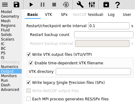
3.6.9. Select output options
Select the
OutputpaneOn the
Basicsub-pane, check theWrite VTK output files (VTU/VTP)checkbox
Select the
VTKsub-paneCreate a new output by clicking the
buttonOn the “select region” dialog, select “particle data” from the
output typedrop-down menuSelect the “Background IC” region from the list to save particle data over the entire domain
Click
OKto create the outputChange the
Write intervalto0.01secondsSelect the
DiameterandTranslational velocitycheck-boxes
3.6.10. Change run parameters
On the Run pane:
Change the
Stop Timeto2.0secondsChange the
Time stepto1e-3secondsChange the
Maximum time stepto1e-2seconds
3.6.11. Run the project
Save project by clicking
 button
Run the project by clicking the
 button
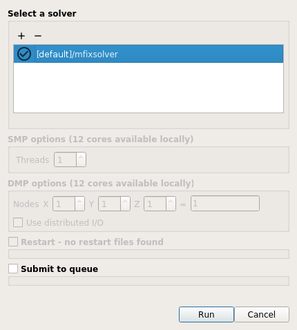
On the
Rundialog, select the default solverClick the
Runbutton to actually start the simulation
3.6.12. View results
Results can be viewed, and plotted, while the simulation is running.
Create a new visualization tab by pressing the
in the upper
right hand corner.Select an item to view, such as plotting the time step (dt) or click the
VTKbutton to view the vtk output files.
