3.21. SMS meshing workflow, cyclone, Discrete Element Model (DEM)¶

This tutorial shows how to use the new meshing workflow, called SMS (Segregated Mesher/Solver). The SMS workflow breaks the CFD workflow into two major steps: Mesher and Solver modes. Each mode of operation is performed in a separate tab in the GUI.

During the Meshing step, the user focuses on generating the mesh and verifies it is appropriate before moving on to the Solver setup. Only three panes are available during Meshing: Geometry, Regions, and Mesh. Once the mesh is generated it must be accepted (after inspection) to unlock the other panes, and move to the second step (Solver mode). The solver mode allows to set all other model settings, and run the MFiX solver to obtain and visualize the simulation results.

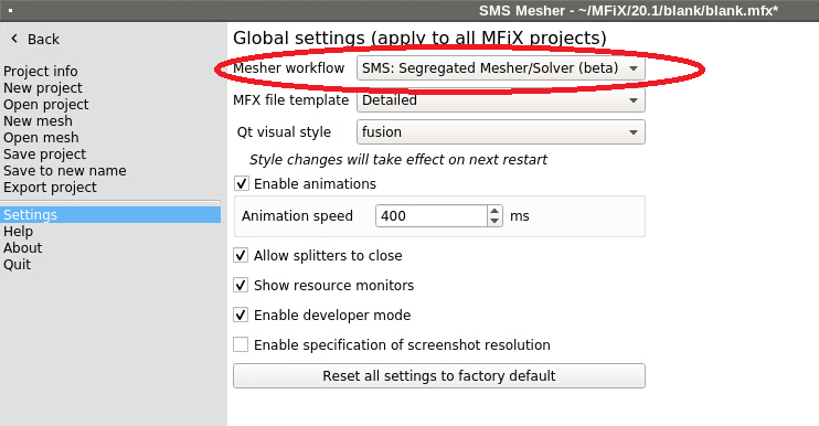
The SMS workflow is currently available as a beta testing feature, and can be turned on from the settings menu (select SMS: Segregated Mesher/Solver (beta) from the Mesher workflow drop down list). The blank template will automatically prompt the user to use the SMS workflow and users are encouraged to try it and provide feedback to the development team.

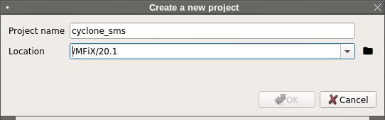
3.21.1. Create a new project¶

On the main menu click on the New button.
Create a new project by double-clicking on “Blank” template.
Enter a project name (say ‘cyclone_sms’ and browse to a location for the new project.

If you have not switched to SMS workflow, you will be prompted to switch. Accept SMS mode.

We are now starting a new project in SMS workflow. There are two tabs in the GUI to setup and run the simulation. The Mesher tab is where the mesh is setup and generated. The Modeler tab is where the rest of the settings and the simulation are performed. The Modeler tab is initially locked until the mesh has been generated and accepted. Running the MFiX solver is also not allowed until the mesh has been generated. At run time, the solver will read the mesh and proceed with the CFD solution.

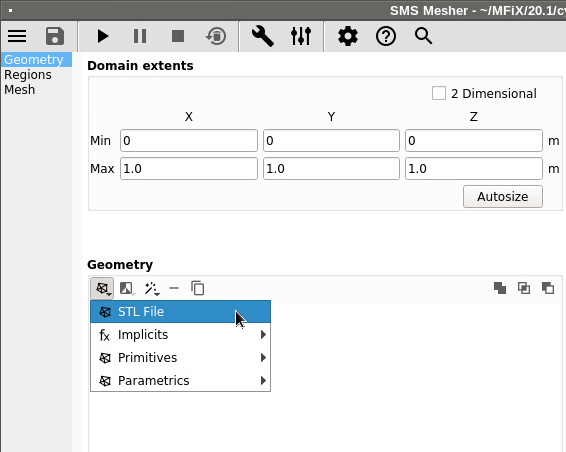
3.21.2. Import the geometry¶

We will use an STL file as the geometry input. Download the file here

Go to the Geometry pane:

Choose STL file as the geometry input.

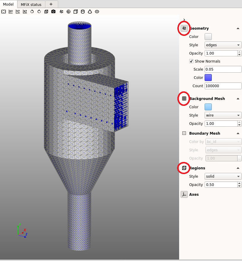
Navigate to where you downloaded cyclone.stl, select it and answer Yes when prompted to copy the file to the project directory.
Verify the STL normals are pointing in the right direction. In the model window, show the Geometry, hide the Background mesh, hide the Regions (visibility is toggled by clicking on each icon). Set the Geometry style to edges, opacity to 1.0, check the Show normals box, set the Scale to 0.05, set count to 10,000 (to show all normals).

The normal vectors should point towards the fluid region (here towards the inside of the cyclone). For internal flows, the tips of the arrows are generally not visible, except through openings in the STL geometry. Openings in the STL geometry are allowed as long as they are outside of the domain extents.

Note

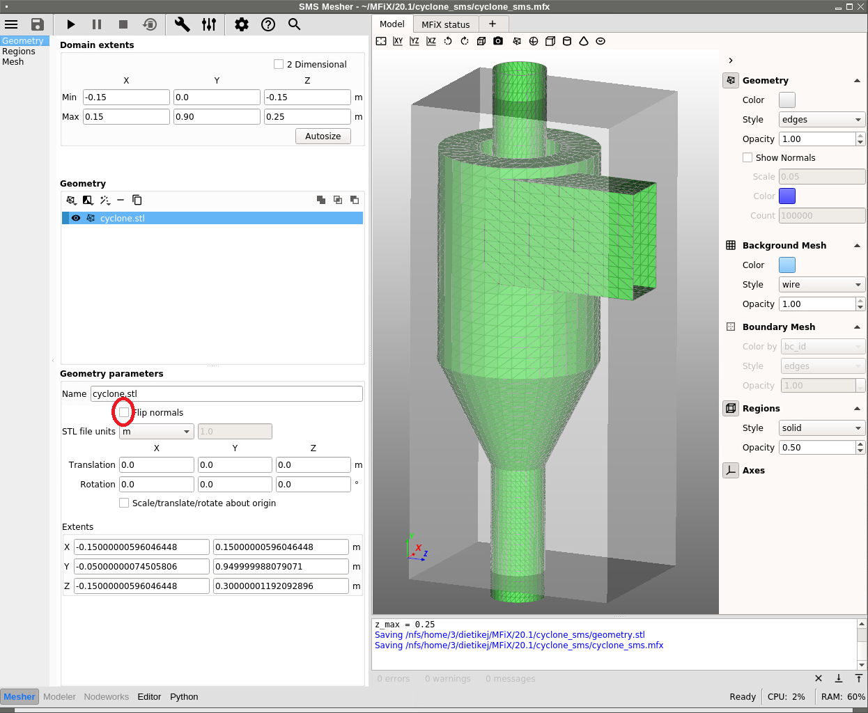
When the normals are pointing in the wrong direction, they can be flipped in the Geometry parameters. Check the Flip normals box and notice the difference in the Model view. Uncheck the box since the original STL file was correctly oriented.

Toggle the Region visibility back on.
In Domain extent, click on Autosize, and adjust the following:
- Enter 0.0 for the Min Y value.
- Enter 0.9 for the Max Y value.
- Enter 0.25 for the Max Z value.

Note that the cyclone inlet and outlets extend beyond the domain extents. This is intentional, as it usually provides a cleaner intersection and easier way to define boundary conditions regions when they are aligned with the domain box (planes along x=xmin, x=xmax etc.).

Save the project by clicking the button.

3.21.3. Create boundary conditions regions¶

Here, we need to define the mesh boundaries. Boundaries include the cyclone wall (curved surface defined by the STL geometry), and the inlet and outlets, defined along the domain outer box (plane boundaries). A boundary condition type must be defined, but it will be possible to change it later (in Modeler Tab). The actual boundary conditions (like the inlet velocity, or outlet pressure) do not need to be set at this point.

Go to the Regions pane:

There is already a Background IC that is predefined in the Blank template. We can ignore it for now.
Click the (top) button to create a new region to be used by pressure outflow boundary condition.
Select Pressure outflow in the Boundary type drop down menu.
Enter a name for the region in the Name field (“Top outlet”).
Change the region color to blue.
Adjust the From/To coordinates in the x-direction: From -0.07 to 0.07.
Adjust the From/To coordinates in the z-direction: From -0.07 to 0.07.
Click the (bottom) button to create a new region to be used by another pressure outflow boundary condition.
Select Pressure outflow in the Boundary type drop down menu.
Enter a name for the region in the Name field (“Bottom outlet”).
Change the region color to yellow.
Adjust the From/To coordinates in the x-direction: From -0.07 to 0.07.
Adjust the From/To coordinates in the z-direction: From -0.07 to 0.07.
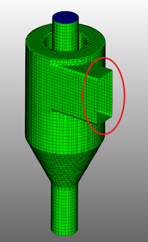
Click the (front) button to create a new region to be used by mass inflow boundary condition.
Select Mass inflow in the Boundary type drop down menu.
Enter a name for the region in the Name field (“Front inlet”).
Change the region color to red.
Adjust the From/To coordinates in the x-direction: From xmin to -0.025.
Adjust the From/To coordinates in the y-direction: From 0.55 to 0.80.
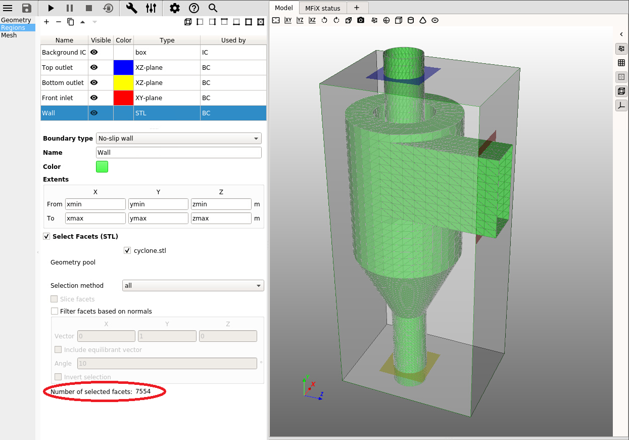
Click the (all) button to create a new region that covers the entire domain to be used for the wall boundary condition.
Select No-slip wall in the Boundary type drop down menu.
Enter a name for the region in the Name field (“Wall”).
Change the region color to green.
Check Select facets (STL) and cyclone.stl, use all for the selection method. You should see that there are 7554 facets selected.

Note

The pressure outlet and mass inflow boundaries are located along the domain box. They are defined as rectangular 2D regions and must overlap the actual boundary areas (intersection of the STL file with the box planes). The exact boundary area will be computed automatically when preprocessing is performed. Since there is only one boundary condition on the top, bottom and front planes, we could also have used the entire planes instead of adjusting the region coordinates.

Save the project by clicking the button.

3.21.4. Setup the mesh¶

Go to the Mesh pane, Background sub-pane:

Enter 25 for the x cell value.
Enter 70 for the y cell value.
Enter 33 for the z cell value.

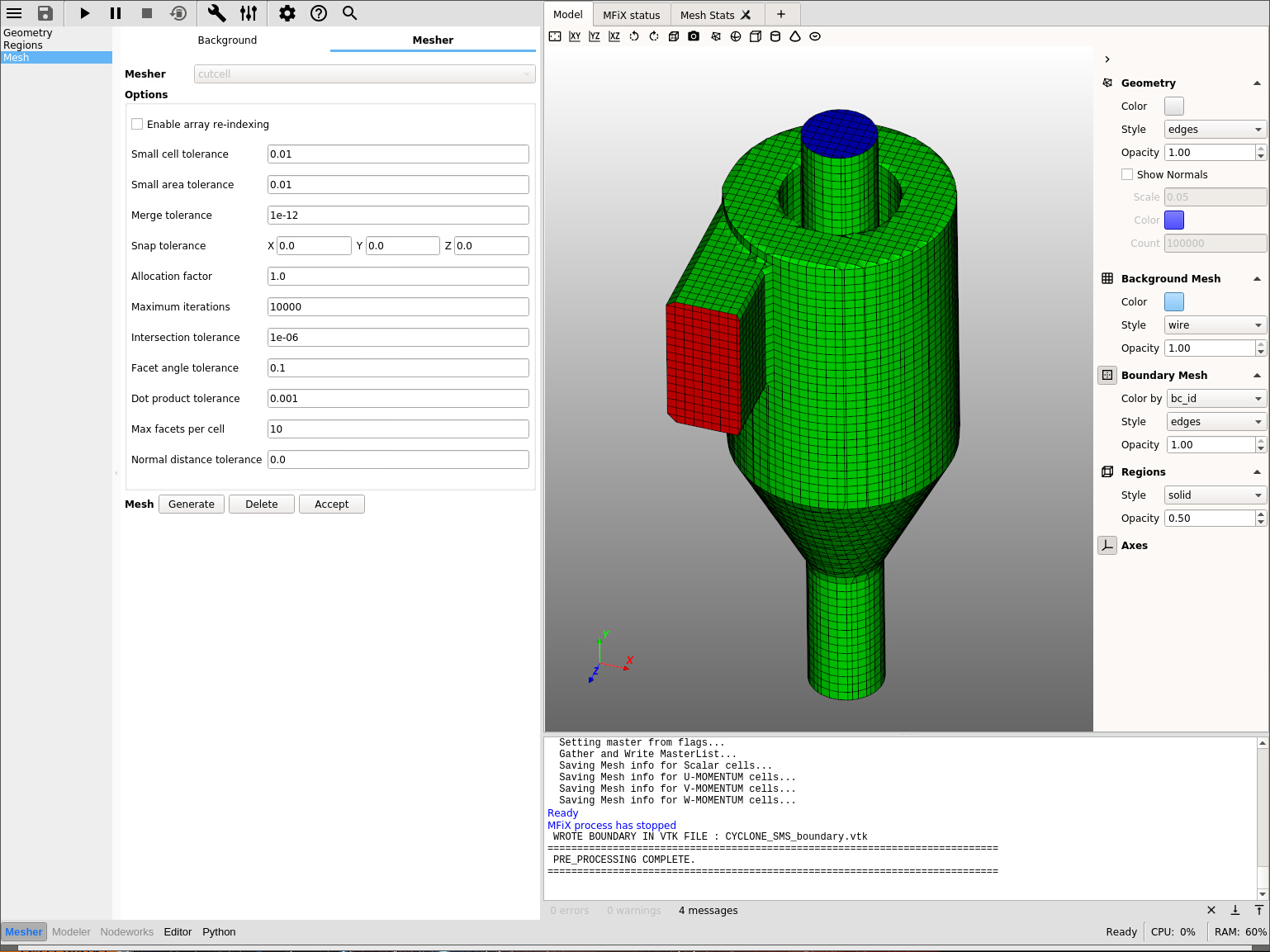
Go to the Mesh pane, Mesher sub-pane:

Keep all default settings and click Generate. Select the default solver, and click Run
Look at the console output to verify the mesh generation completed successfully.
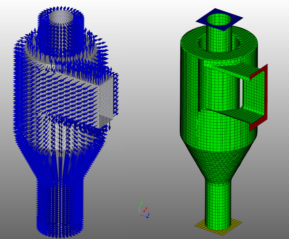
In the Model view - hide the Geometry, Background mesh and Regions, - show the Boundary mesh - set Color by to bc_id, - set Style to edges and opacity to 1.0.
The boundary mesh should look like a closed surface with colors matching the boundary conditions regions.

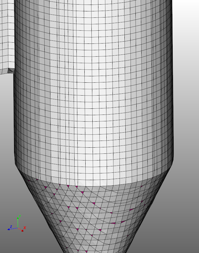
Color the boundary mesh by small_cell. This will show small cells, as defined by the small cell tolerance. The default value of 0.01 means a cut cell is considered small if its volume is below 0.01 times the volume of the corresponding standard, uncut cell. These small cells will be removed from the computation. Having a Small cell tolerance set to 0.0 will keep all small cells and this may lead to numerical stiffness and loss of convergence.

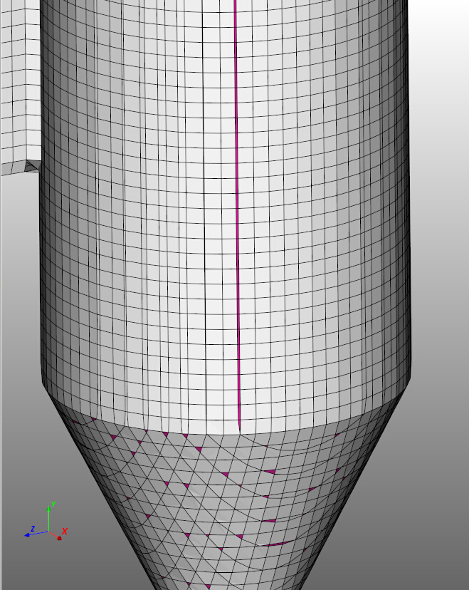
Having a few small cells is usually acceptable. In some cases it is possible to reduce the number of small cells by adjusting some cut cell parameters. Increase the Snap tolerance to 0.1 in the x, y, and z-direction. Generate the mesh again, and visualize the small cells. The vertical column of small cells was eliminated.

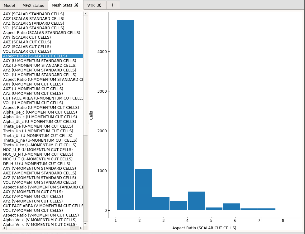
Mesh colored by small cell, with snapping

Mesh statistics (histogram) can be viewed in the Mesh Stats viewport. Various quantities are available. For example the aspect ratio of cut cells is between 1 and 8, with most aspect ratios between 1 and 2. This is acceptable.

After inspection, the mesh is deemed acceptable and we can move to the second step (Solver mode). Click Accept. This will unlock the Modeler tab.

Note

Optional but recommended: To see examples of unacceptable meshes, try the following:

Go back to the Geometry pane, and flip the normals. This will incorrectly orient the STL file. This is a common error when importing STL files. Generate the mesh and visualize the boundary mesh. Having an open surface and boundaries inside-out is an indication that the normals are not properly oriented. The mesh should not be accepted.

Uncheck the Flip normals box in the Geometry pane to get correct orientation. Go to the Region pane, and select the Front inlet region in the region table and set the Boundary type to None. Save the project and generate the mesh. The boundary mesh will look like an open surface, this is an indication a boundary condition is missing. The mesh should not be accepted.

Remember to set the Front inlet region boundary type to Mass inflow again before continuing. Generate the mesh, inspect it and accept it before moving to the Modeler tab.

3.21.5. Model settings¶

Switch to the Modeler tab (second tab at the bottom left corner of the GUI).

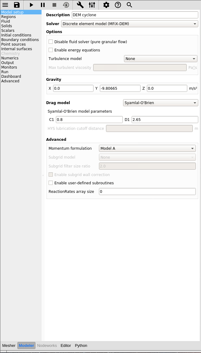
On the Model pane, enter a descriptive text in the Description field.
Select “Discrete Element Model (MFiX-DEM)” in the Solver drop-down menu.
Keep all other settings at their default values.

3.21.6. Regions settings¶

We already have the Background_IC region that is predefined. We will use it to initialize the flow field. We have defined all Boundary Condition regions during the meshing step. There are no other regions that need to be defined in this tutorial. We will re-use Background_IC region for the VTK output file.

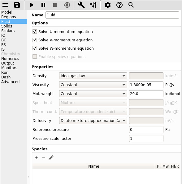
3.21.7. Fluid settings¶

Change Density to Ideal gas law.
Keep all other settings at their default values.

3.21.8. Solids settings¶

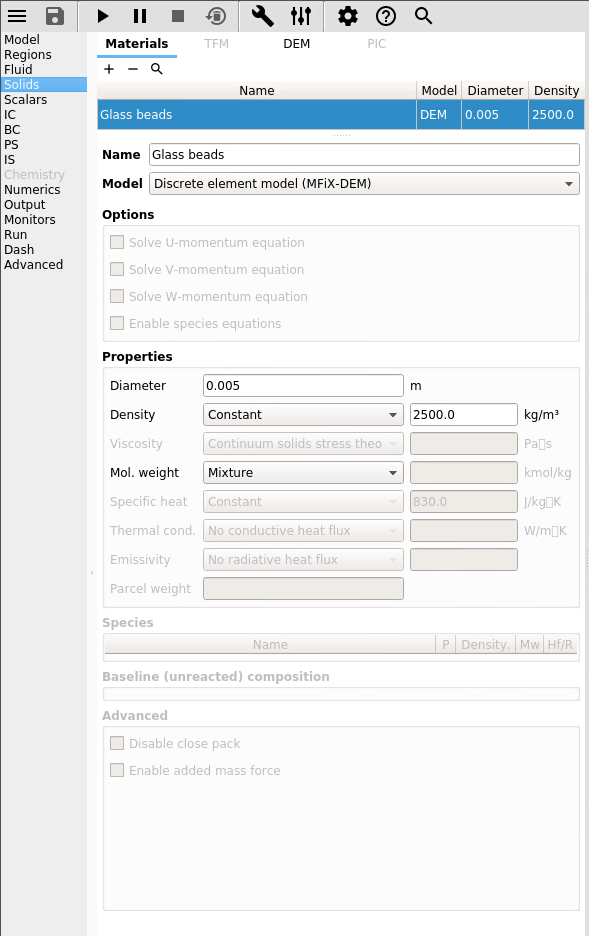
On the Solids pane, Materials sub-pane:

Click the button to create a new solid.
Enter a descriptive name in the Name field (“Glass beads”).
Verify the solids model is already set to “Discrete Element Model (MFiX-DEM)”.
Enter the particle diameter of 0.005 m in the Diameter field.
Enter the particle density of 2500 kg/m³ in the Density field.

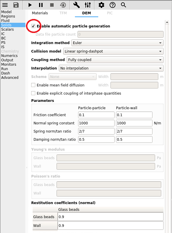
Select the Solids pane, DEM sub-pane.
Check the Enable automatic particle generation checkbox. Although we will start with an empty cyclone, this setting is necessary so we don’t attempt to read initial particle location from particle_input.dat.
Keep all other settings at their default values.

3.21.9. Initial Conditions settings¶

On the Initial conditions pane:

There is already a pre-defined “Background IC” region. This will initialize the entire flow field with air at rest.
Keep all settings at their default values.

3.21.10. Boundary Conditions settings¶

On the Boundary conditions pane:

The Top outlet and Bottom outlet Boundary Conditions are already set to atmospheric pressure. No changes are needed.
The Wall Boundary Conditions is already set to No-slip wall. No changes are needed.
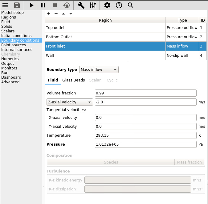
Select the Front Inlet region from the list.
- In the Glass beads tab: set the Volume fraction to 0.01, and Z-axial velocity to -2.0.
- In the Fluid tab, verify the Gas volume fraction was automatically set to 0.99 and set the Z-axial velocity to -2.0.
Keep all other settings at their default values.

3.21.11. Numerics settings¶

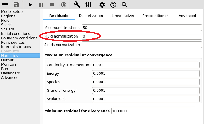
On the Numerics pane:

Set the Fluid normalization to 0.0.
Keep all other settings at their default values.

3.21.12. Output settings¶

On the Output pane:

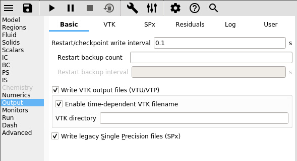
On the Basic sub-pane, check the Write VTK output files (VTU/VTP) checkbox.

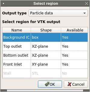
Select the VTK sub-pane.
Create a new output by clicking the button.
Select “Particle Data” from the ‘Output type’ drop-down menu.
Select the “Background IC” region from the list to save all the particle data.
Click OK to create the output.

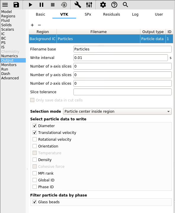
Enter a base name for the *.vtu files in the Filename base field (“Particles”).
Change the Write interval to 0.01 seconds.
Select the Diameter and Translational Velocity checkboxes.

3.21.13. Run settings¶

Save the project by clicking the save button.

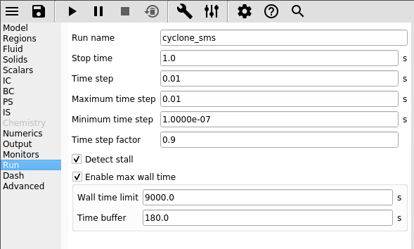
On the Run pane:

Set Stop time to 1.0.
Set Time step to 0.01.
Set Maximum time step to 0.01.
Keep all other settings at their default values.

3.21.14. Run the simulation¶

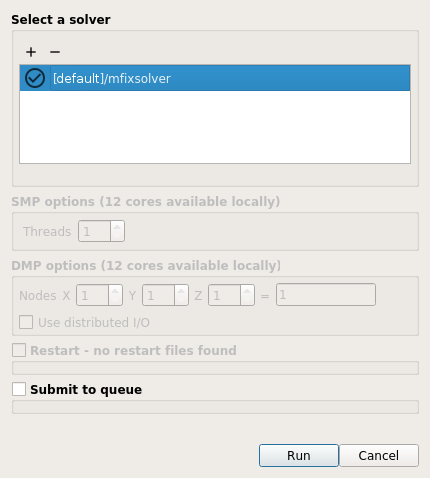
Run the project by clicking the button.
On the Run dialog, select the executable from the combo-box.
Click the Run button to actually start the simulation.

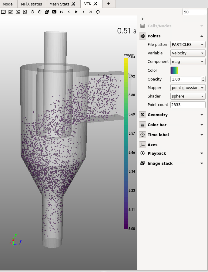
3.21.15. View results¶

Results can be viewed, and plotted, while the simulation is running.

Create a new visualization tab by pressing the next to the Model tab.
Click the 3D view button to view the vtk output files.
On the VTK results tab, the visibility and representation of the *.vtk files can be controlled with the menu on the side.
Change frames with the , , , and buttons.
Click the button to play the available vtk files.
Change the playback speed under the section on the sidebar.