3.23. Procedural geometry¶

This tutorial shows how to use procedural shapes to define geometry. This capability was introduced in the 21.1 release.

Simple shapes (cylinder and bends) will be defined and combined to create the geometry. Each shape is controlled by parameters. Filters are applied to the shapes to transform (scale, translate, rotate) the geometry, or flip the normal vector orientation (internal vs external flow). Boolean operations are used to combine the shapes.

The primary focus of this tutorial is to build the geometry. This is done in SMS mode (see SMS meshing workflow tutorial for more details).

3.23.1. Create a new project¶

On the main menu click on the New button.
Create a new project by double-clicking on “Blank” template.
Enter a project name and browse to a location for the new project.

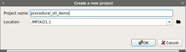
If you have not switched to SMS workflow, you will be prompted to switch. Accept SMS mode.

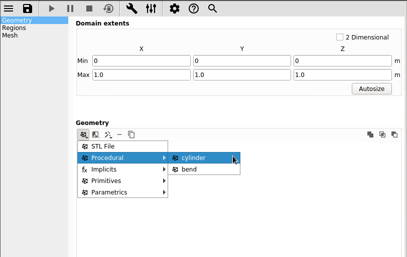
3.23.2. Create the geometry¶

First, create a cylinder:

Go to the Geometry pane and click the add button to add geometry:

Choose -> Procedural > Cylinder as the geometry input (named cylinder).

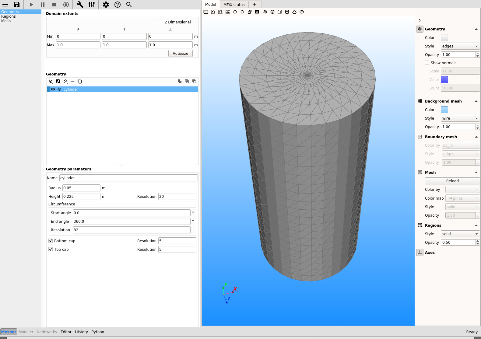
Enter the cylinder’s parameters:
- Radius = 0.05 m, Height = 0.225 m, Resolution = 20
- Start angle= 0 deg, end angle = 360 deg, resolution = 32
- Check the Bottom cap and Top cap check boxes and set the resolution to 5 for both caps.

Save the project by clicking the button.

Next, create a bend:

Go to the Geometry pane:

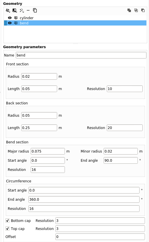
Choose -> Procedural > Bend as the geometry input (named “bend”).
Enter the bend’s parameters:
- Front section: Radius = 0.02 m, Length = 0.05 m, Resolution = 10
- Back section: Radius = 0.05 m, Length = 0.25 m, Resolution = 20
- Bend section: Major radius = 0.075 m, Minor radius = 0.02 m, Start angle= 0 deg, end angle = 90 deg, resolution = 16
- Circumference: Start angle= 0 deg, end angle = 360 deg, resolution = 16
- Check the Bottom cap and Top cap check boxes and set the resolution to 3 for both caps. Leave Offset = 0

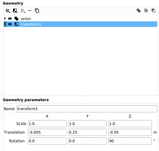
Rotate and translate the bend:
- Select the bend (named bend)
- Add a filter: -> transform
- Set a Translation of 0.025 m in the X-direction, 0.15 m in the Y-direction, and 0.05 m in the Z-direction.
- Rotate -90 deg in the Z-direction.

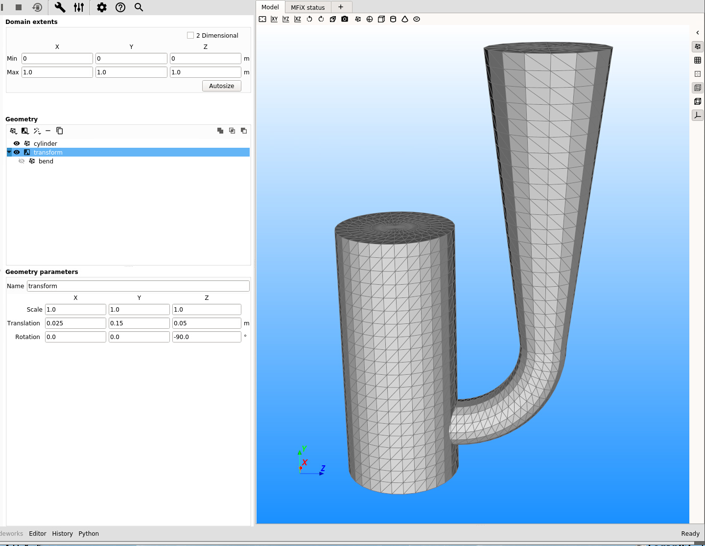
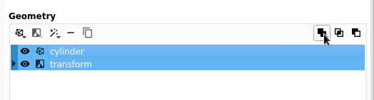
Combine the cylinder and the bend (union):
- Select the cylinder (named cylinder)
- While holding the ctrl key, select the transformed bend (named transform)
- Press the button

Save the project by clicking the button.

Next, create another bend:

Go to the Geometry pane:

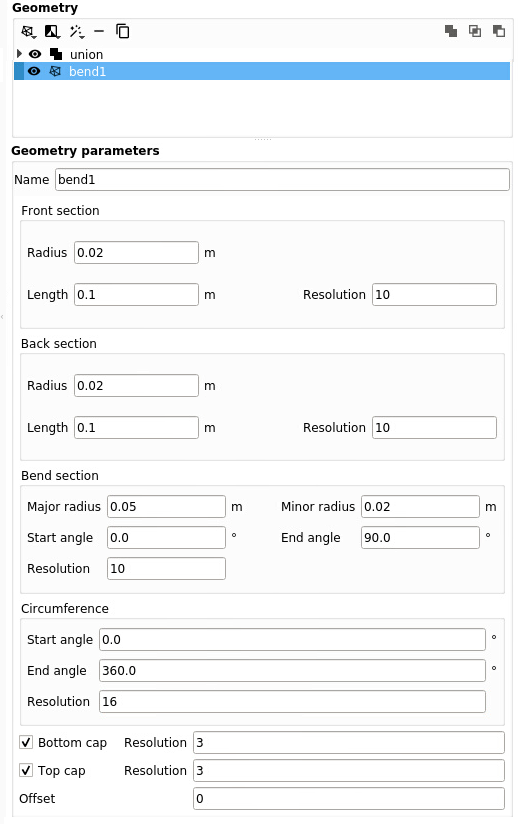
Choose -> Procedural > Bend as the geometry input (named bend1).
Enter the bend’s parameters:
- Front section: Radius = 0.02 m, Length = 0.1 m, Resolution = 10
- Back section: Radius = 0.02 m, Length = 0.1 m, Resolution = 10
- Bend section: Major radius = 0.05 m, Minor radius = 0.02 m, Start angle= 0 deg, end angle = 90 deg, resolution = 10
- Circumference: Start angle= 0 deg, end angle = 360 deg, resolution = 16
- Check the Bottom cap and Top cap check boxes and set the resolution to 3 for both caps. Leave Offset = 0

Rotate and translate the bend:
- Select the bend (named bend1)
- Add a filter: -> transform
- Set a Translation of -0.005 m in the X-direction, 0.25 m in the Y-direction, and -0.05 m in the Z-direction.
- Rotate 90 deg in the Z-direction.

Combine the bend and the previous geometry (union):
- Select the transformed bend (named transform1)
- While holding the ctrl key, select the previous geometry (named union)
- Press the button. This will create a new union1 geometry.
Save the project by clicking the button.

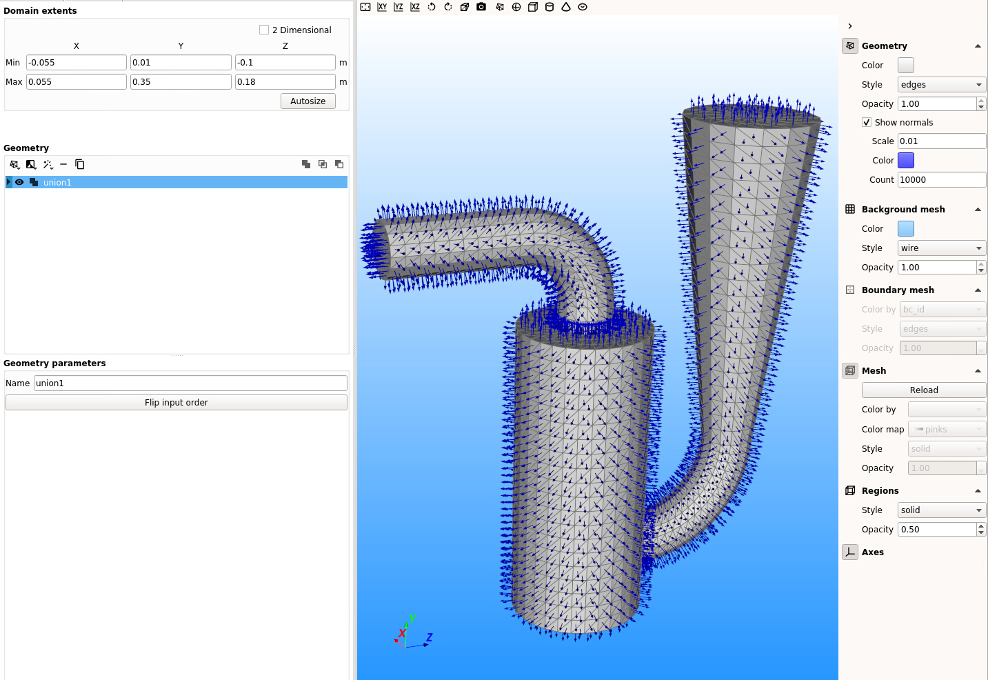
3.23.3. Check the geometry orientation¶

Visualize and flip the orientation (normal vectors) of the geometry:

In the model window, show the Geometry, hide the Background mesh, Hide the Regions (visibility is toggled by clicking on each icon). Set the Geometry style to edges, opacity to 1.0, check the Show normals box, set the Scale to 0.01, set count to 10,000 (to show all normals).

The normal vectors must point towards the fluid region (here towards the inside of the geometry). However we see that the normals point in the opposite direction (outwards the fluid region). This means we need to flip the normals to correct the orientation.

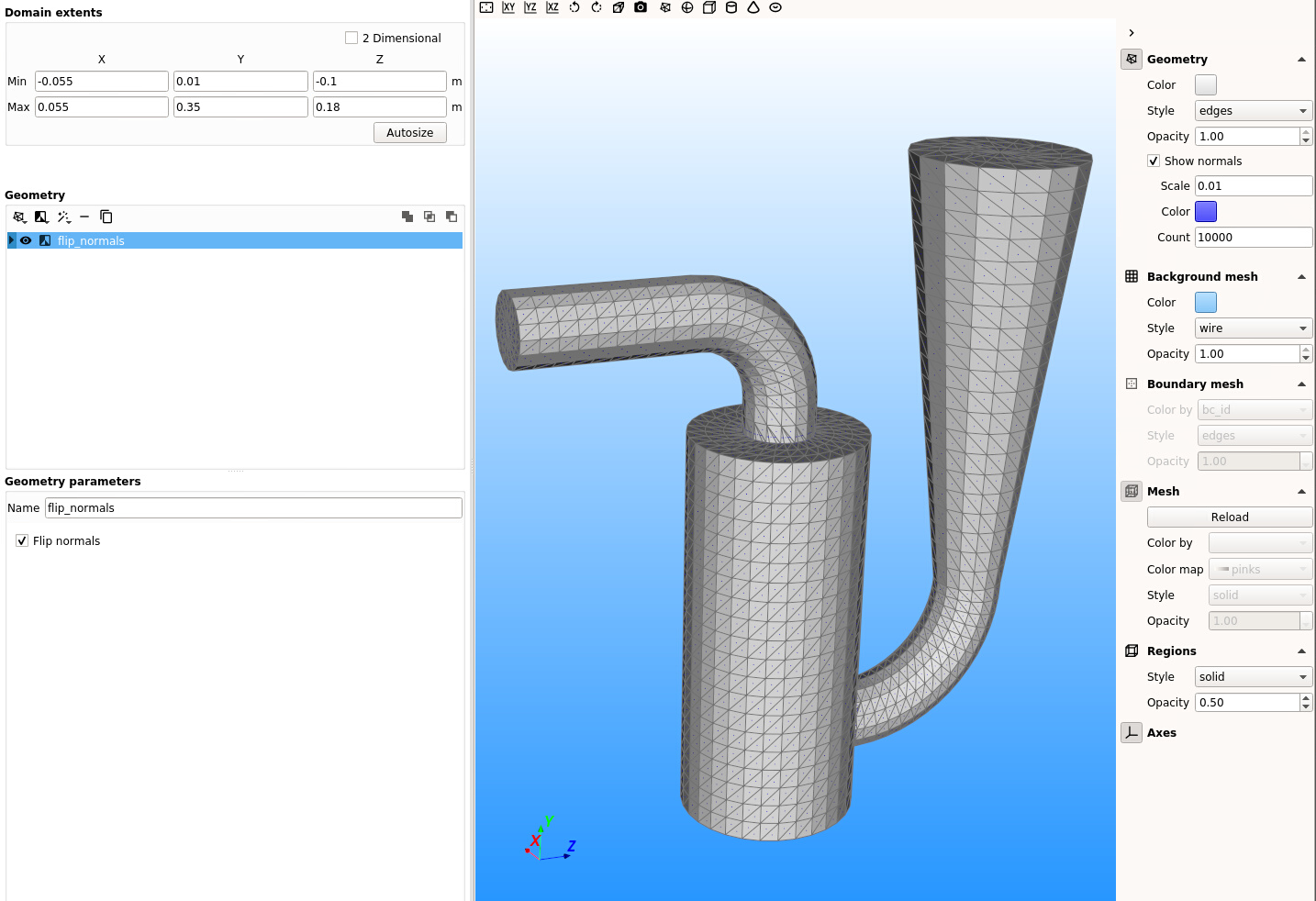
Select the union1 geometry,
Add a filter: -> flip normals. Now the vectors point towards the fluid region. The tips of the arrows are not visible, but we can see the origin (shown as a dot at the center of each face).

Save the project by clicking the button.
Toggle the Region visibility back on.
In Domain extent, enter the following:
- X-direction: Min = -0.055 m, Max = 0.055 m.
- Y-direction: Min = 0.01 m, Max = 0.35 m.
- Z-direction: Min = -0.1 m, Max = 0.18 m.

Note that the inlets and outlet extend beyond the domain extents. This is intentional, as it usually provides a cleaner intersection and easier way to define boundary conditions regions when they are aligned with the domain box (planes along x=xmin, x=xmax etc.).

Save the project by clicking the button.

3.23.4. Create boundary conditions regions¶

Go to the Regions pane:

There is already a Background IC that is predefined in the Blank template. We can ignore it for now.
Click the (top) button to create a new region to be used by a mass inflow boundary condition.
Select Mass inflow in the Boundary type drop down menu.
Enter a name for the region in the Name field (“top inlet”).
Change the region color to red.
Click the (bottom) button to create a new region to be used by another mass inflow boundary condition.
Select Mass inflow in the Boundary type drop down menu.
Enter a name for the region in the Name field (“bottom inlet”).
Change the region color to pink.
Click the (back) button to create a new region to be used by pressure outlet boundary condition.
Select Pressure outflow in the Boundary type drop down menu.
Enter a name for the region in the Name field (“outlet”).
Change the region color to yellow.
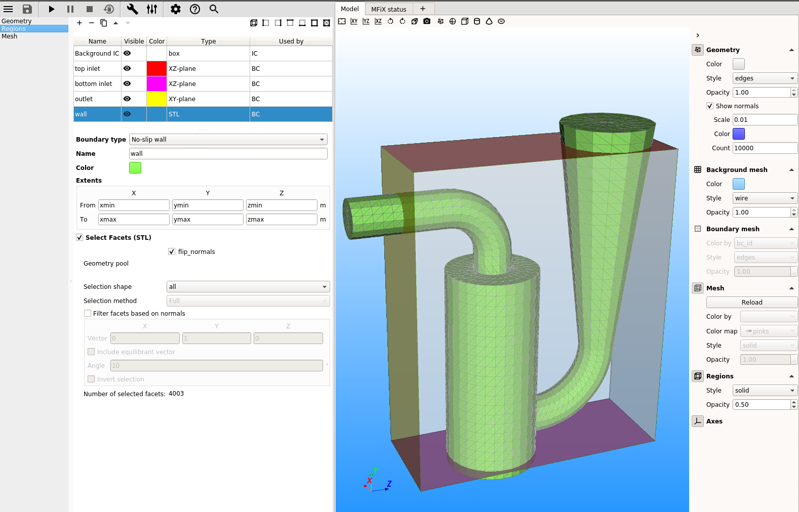
Click the (all) button to create a new region that covers the entire domain to be used for the wall boundary condition.
Select No-slip wall in the Boundary type drop down menu.
Enter a name for the region in the Name field (“wall”).
Change the region color to green.
Check Select facets (STL) and flip_normals, use all for the selection method. You should see that there are 4003 facets selected.

Note

The pressure outlet and mass inflow boundaries are located along the domain box. They are defined as rectangular 2D regions and must overlap the actual boundary areas (intersection of the STL file with the box planes). The exact boundary area will be computed automatically when preprocessing is performed.

Click the (all) button to create a new region that will be used as initial condition region. This is not needed to generate the mesh, but will be used later when setting up the simulation.
Leave the Boundary type as None.
Enter a name for the region in the Name field (“init bed”).
Change the region color to black.
Set the Y-extent form ymin to 0.15 m.
Save the project by clicking the button.

3.23.5. Setup the mesh¶

Go to the Mesh pane, Background sub-pane:

Enter 15 for the x cell value.
Enter 35 for the y cell value.
Enter 30 for the z cell value.

Go to the Mesh pane, Mesher sub-pane:

Set the Facet angle tolerance to 0.0 deg. (The geometry unions have created elongated triangles we need to keep).
Click Generate.
Look at the console output to verify the mesh generation completed successfully.
In the Model view, - hide the Geometry, Background mesh and Regions - show the Boundary_Mesh - set Color by to bc_id, - set Style to edges and opacity to 1.0.
The Boundary_Mesh should look like a closed surface with colors matching the boundary conditions regions.

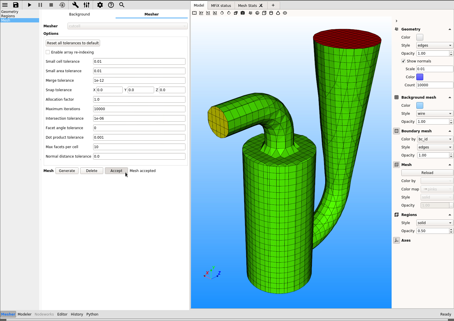
After inspection, the mesh is deemed acceptable and we can move to setting up the simulation (Solver mode). Click Accept. This will unlock the Modeler tab.

3.23.6. Model settings¶

Switch to the Modeler tab (second tab at the bottom left corner of the GUI).

On the Model pane, enter a descriptive text in the Description field.
Select “Discrete Element Model (MFiX-DEM)” in the Solver drop-down menu.
Keep all other settings at their default values.

3.23.7. Regions settings¶

We already have set all the regions, there is no change required in this pane.

3.23.8. Fluid settings¶

Change Density to Ideal gas law.
Keep all other settings at their default values.

3.23.9. Solids settings¶

On the Solids pane, Materials sub-pane:

Click the button to create a new solid.
Verify the solids model is already set to “Discrete Element Model (MFiX-DEM)”.
Enter the particle diameter of 0.005 m in the Diameter field.
Enter the particle density of 2700 kg/m³ in the Density field.
Select the Solids pane, DEM sub-pane.
Check the Enable automatic particle generation checkbox.
Keep all other settings at their default values.

3.23.10. Initial conditions settings¶

On the Initial conditions pane:

There is already a Background IC region that initializes the entire domain as stagnant air. We only need to add solids at the bottom.
Create a new initial condition region by clicking the button.
Select the init bed region, go to the Solid 1 tab and enter 0.5 for the volume fraction.

3.23.11. Boundary conditions settings¶

On the Boundary conditions pane:

Select the top inlet region. In the Solids 1 tab, enter 0.2 for the volume fraction and -0.2 for the Y-axial velocity.
Select the bottom inlet region. Stay on the Fluid tab, enter 4.0 for the Y-axial velocity.
The outlet Boundary Conditions is already set to atmospheric pressure. No changes are needed.
The Wall Boundary Conditions is already set to No-slip wall. No changes are needed.

3.23.12. Numerics settings¶

On the Numerics pane:

On the Residual pane: set the Fluid normalization to 0.0 and the fluid pressure correction scale factor to 1.0
On the Preconditioner tab, set the preconditioner to None for all equations.

3.23.13. Output settings¶

On the Output pane:

On the Basic sub-pane, check the Write VTK output files (VTU/VTP) checkbox.
Select the VTK sub-pane.
Create a new output by clicking the button.
Select “Particle Data” from the ‘Output type’ drop-down menu.
Select the “Background IC” region from the list to save all the particle data.
Click OK to create the output.
Enter a base name for the *.vtu files in the Filename base field (“Particles”).
Change the Write interval to 0.01 seconds.
Select the Diameter and Translational Velocity checkboxes.

3.23.14. Run settings¶

Save the project by clicking the save button.

On the Run pane:

Set Stop time to 1.0.
Set Time step to 0.001.
Set Maximum time step to 0.01.
Keep all other settings at their default values.

3.23.15. Run the simulation¶

Run the project by clicking the button.
On the Run dialog, select the executable from the combo-box.
Click the Run button to actually start the simulation.

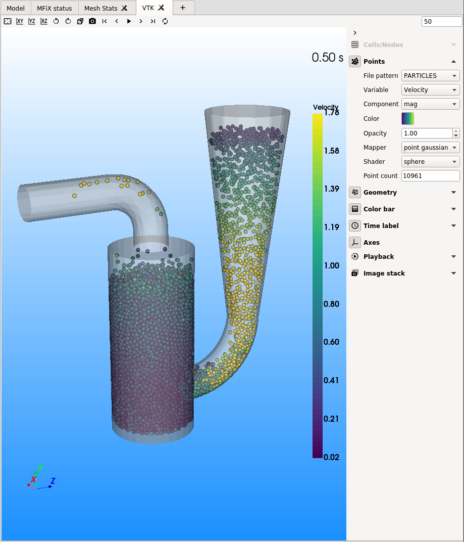
3.23.16. View results¶

Results can be viewed, and plotted, while the simulation is running.

Create a new visualization tab by pressing the next to the Model tab.
Click the 3D view button to view the vtk output files.
On the VTK results tab, the visibility and representation of the *.vtk files can be controlled with the menu on the side.
Change frames with the , , , and buttons.
Click the button to play the available vtk files.
Change the playback speed under the section on the sidebar.