3.5. Three-dimensional fluidized bed¶

This tutorial shows how to create a three dimensional fluidized bed simulation using the two-fluid model (TFM) and the discrete element model (DEM). The model setup is:

Property	Value
geometry	10 cm diameter x 40 cm
mesh	20 x 60 x 20
solid diameter	200 microns (\(200 \times 10^{-6}\) m)
solid density	2500 kg/m²
gas velocity	0.25 m/s
temperature	298 K
pressure	101325 Pa

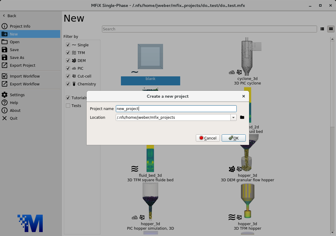
3.5.1. Create a new project¶

On the main menu, select New project
Create a new project by double-clicking on “Blank” template.
Enter a project name and browse to a location for the new project.
When prompted to enable SMS workflow, answer No, we will use the standard workflow for this tutorial.

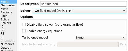
3.5.2. Select model parameters¶

On the Model pane:

Enter a descriptive text in the Description field
Select “Two-Fluid Model (MFiX-TFM)” in the Solver drop-down menu.

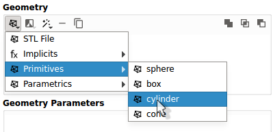
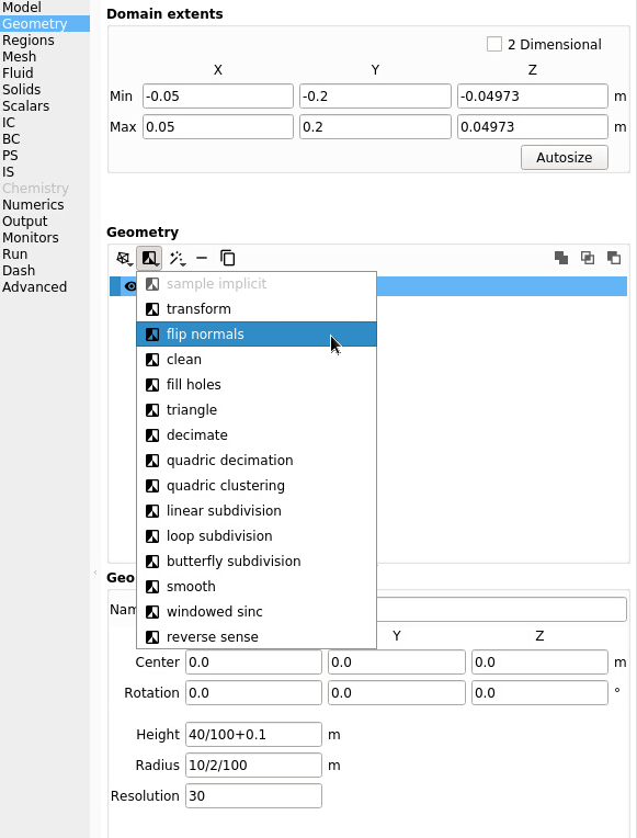
3.5.3. Enter the geometry¶

On the Geometry pane:

Create the cylindrical geometry by pressing the Add Geometry button -> Primitives -> cylinder

Enter 40/100 meters for the cylinder height
Enter 10/2/100 meters for the cylinder radius
Enter 30 for the cylinder resolution
Press the autosize button to fit the domain extents to the geometry
Extend the height of the cylinder by adding 0.1 meters. This will hang the stl file outside of the domain, allowing for a sharp and clean cut.
Flip the normals by clicking the button and selecting the flip normals filter

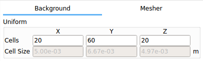
3.5.4. Enter the mesh¶

On the Mesh pane:

On the Background sub-pane

Enter 20 for the x cell value

Enter 60 for the y cell value

Enter 20 for the z cell value

Note

This is a fairly coarse grid for a TFM simulation. After completing this tutorial, try increasing the grid resolution to better resolve the bubbles.

3.5.5. Create regions for initial and boundary condition specification¶

Select the Regions pane. By default, a region that covers the entire domain is already defined. This is typically used to initialize the flow field and visualize the results.

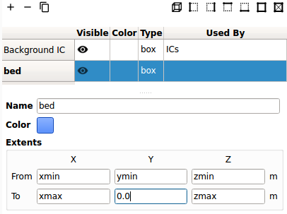
Click the (all) button to create a new region to be used for the bed initial condition.
Enter a name for the region in the Name field (“bed”)
Change the color by pressing the Color button
Enter 0 in the To Y field

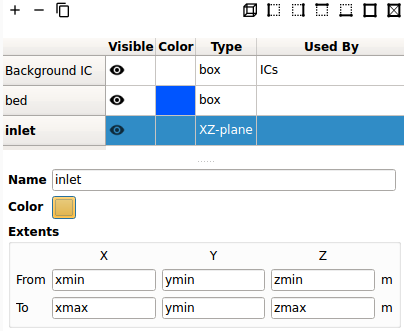
Click the (bottom) button to create a new region to be used by the gas inlet boundary condition.
Enter a name for the region in the Name field (“inlet”)

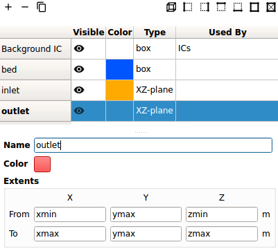
Click the (top) button to create a new region to be used by the pressure outlet boundary condition.
Enter a name for the region in the Name field (“outlet”)

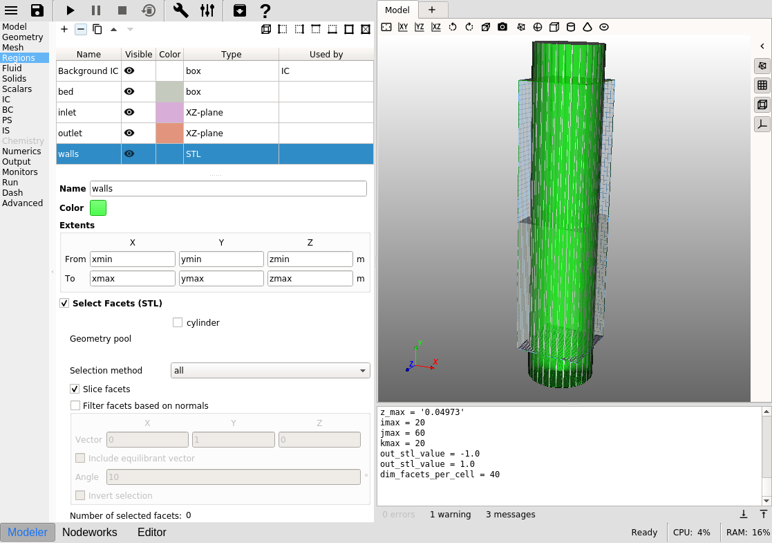
Click the (all) button to create a new region to be used to select the walls.
Enter a name for the region in the Name field (“walls”)
Click the Select facets box. The region type should change from “box” to “STL”.

All the facets of the cylinder should now be selected. Since the cylinder is outside the domain extents, normal cells (i.e. not cut-cells) will be placed at the outlet and inlet. This allows for the standard boundary conditions to be applied.

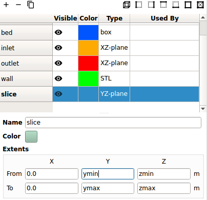
Click the (left) button to create a new region to be used to save a slice of cells at the center of the domain.
Enter a name for the region in the Name field (“slice”)
Enter 0 in the From X and To X fields

3.5.6. Create a solid¶

On the Solids pane:

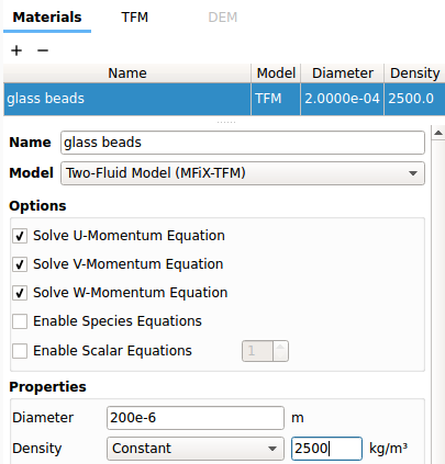
Click the button to create a new solid
Enter a descriptive name in the Name field (“glass beads”)
Accept the radial distribution setting (Carnahan-Starling)
Enter the particle diameter of 200e-6 m in the Diameter field
Enter the particle density of 2500 kg/m² in the Density field

3.5.7. Create Initial conditions¶

On the Initial conditions pane:

Select the already populated “Background” from the region list. This will initialize the entire flow field with air.
Enter 101325 Pa in the Pressure (optional) field
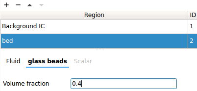
Create a new Initial Condition by pressing the button
Select the region created previously for the bed Initial Condition (“bed” region) and click the OK button.
Select the solid (named previously as “glass beads”) sub-pane and enter a volume fraction of 0.4 in the Volume Fraction field. This will fill the bottom half of the domain with glass beads.

3.5.8. Create Boundary conditions¶

On the Boundary conditions pane:

Create a new Boundary condition by clicking the button
On the Select region dialog, select “Mass Inflow” from the Boundary type drop-down menu
Select the “inlet” region and click OK
On the Fluid sub-pane, enter a velocity in the Y-axial velocity field of 0.25 m/s
Create another Boundary condition by clicking the button
On the Select region dialog, select “Pressure outflow” from the Boundary type combo-box
Select the “outlet” region and click OK

Note

The default pressure is already set to 101325 Pa, no changes need to be made to the outlet boundary condition.

Create another Boundary condition by clicking the button
On the Select region dialog, select “No Slip Wall” from the Boundary type combo-box
Select the “wall” region and click OK

3.5.9. Change numeric parameters¶

On the Numerics pane, Residuals sub-pane:

Enter 0 in the Fluid Normalization field.

3.5.10. Select output options¶

On the Output pane:

On the Basic sub-pane, check the Write VTK output files (VTU/VTP) checkbox
Select the VTK sub-pane
Create a new output by clicking the button
Select the “Background” region from the list to save all the cell data
Click OK to create the output
Enter a base name for the *.vtu files in the Filename base field
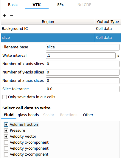
Change the Write interval to 0.01 seconds
Select the Volume fraction, Pressure, and Velocity vector checkboxes on the Fluid tab
Create another output by clicking the button
Select the “Slice” region from the list to save all the cell data
Click OK to create the output
Enter a base name for the *.vtu files in the Filename base field
Change the Write interval to 0.01 seconds
Select the Volume fraction, Pressure, and Velocity vector checkboxes on the Fluid tab

3.5.11. Change run parameters¶

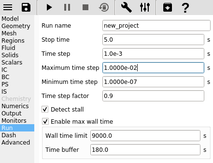
On the Run pane:

Change the Stop time to 1.0 seconds
Change the Time step to 1e-3 seconds
Change the Maximum time step to 1e-2 seconds

3.5.12. Run the project¶

Save project by clicking button
Run the project by clicking the button
On the Run dialog, select the default executable from the list
Click the Run button to actually start the simulation

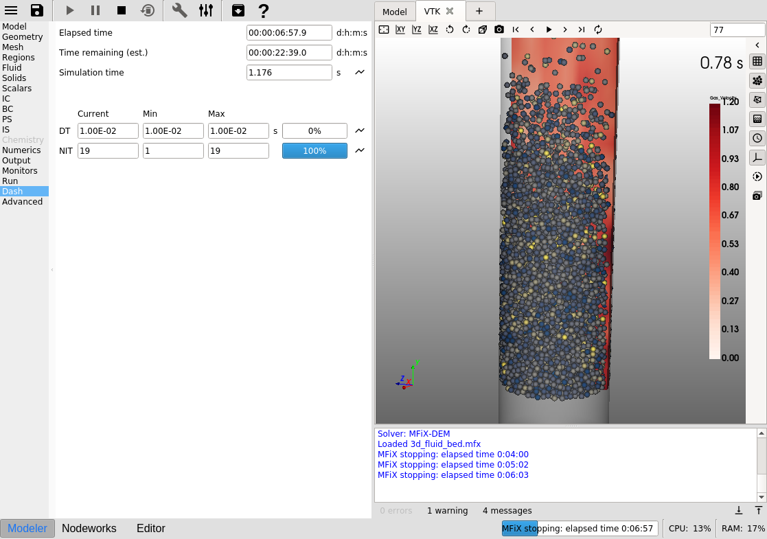
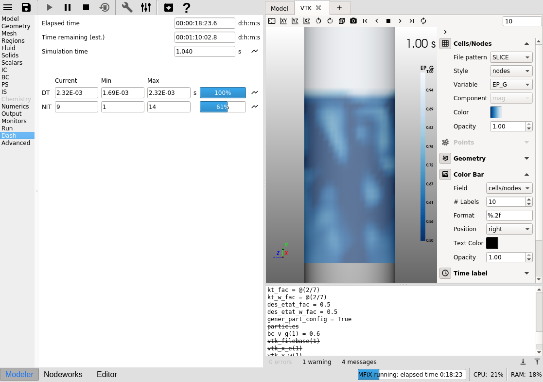
3.5.13. View results¶

Results can be viewed, and plotted, while the simulation is running.

Create a new visualization tab by pressing the next to the Model tab
Select an item to view, such as plotting the time step (dt) or click the 3D view button to view the vtk output files.
On the VTK results tab, the visibility and representation of the *.vtk files can be controlled with the menu on the side.

3.5.14. Convert this project into a 3D DEM simulation¶

Click the button and delete all simulation files.
Close the VTK window
On the Model pane, change the solver to MFiX-DEM
On the Mesh pane, coarsen the grid to 15, 45, and 15 cells in the in the x, y, and z direction, respectfully.

Note

The grid resolution needs to be coarser because we are drastically increasing the particle diameter below. The fluid grid cell size has to be bigger than the particle size.

On the Solids pane, change that particle diameter to 5.0000e-03 to get a more reasonable particle count for tutorial purposes.
On the Solids pane, DEM sub-pane: - check the Enable automatic particle generation - enter a value of 15 in the Search grid partitions, KMAX field.
On the Boundary conditions pane, change the inlet Y-axial velocity to 0.6 m/s
On the Boundary conditions pane, delete the walls boundary condition and re-add it to write the correct wall parameters for the DEM simulation.
On the Output pane, VTK sub-pane:
- Delete the all or Background_IC output
- Create a new output, change the Output type to Particle data and select the Background_IC region.
- Change the write frequency to 0.01
- Select the Diameter and Translational Velocity data
Run the simulation
Create a VTK window to visualize the data. It will automatically show the slice (cell data) and the particles.