3.7. DEM granular flow chutes
This tutorial shows how to create a three dimensional pure granular flow simulation from a series of cylindrical chutes. The model setup is:
Property |
Value |
|---|---|
geometry |
1.75 m x 0.94 m x 0.2 m |
mesh |
20 x 20 x 10 |
solid diameter |
12.5 mm (0.0125 m) |
solid density |
2500 kg/m2 |
temperature |
298 K |
pressure |
101325 Pa |
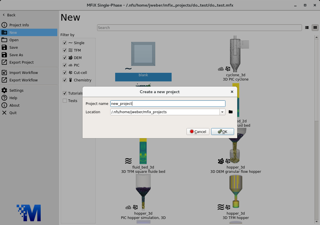
3.7.1. Create a new project
On the main menu, select
New projectCreate a new project by double-clicking on “Blank” template.
Enter a project name and browse to a location for the new project.
When prompted to enable SMS workflow, answer No, we will use the standard workflow for this tutorial.
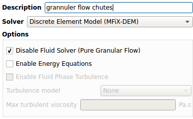
3.7.2. Select model parameters
On the Model pane:
Enter a descriptive text in the
DescriptionfieldSelect “Discrete Element Model (MFiX-DEM)” in the
Solverdrop-down menu.Check the
Disable Fluid Solvercheckbox.
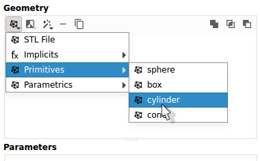
3.7.3. Enter the geometry
On the Geometry pane:
Create the cylindrical geometry by pressing
 ->
-> primitives->cylinderEnter
0.1meters for the cylinder radiusEnter
30for the cylinder resolution
Create another cylindrical geometry by pressing
-> primitives->cylinderEnter
1.2meters for the cylinder heightEnter
0.08meters for the cylinder radiusEnter
30for the cylinder resolution
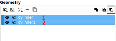
Subtract the smaller radius cylinder from the larger radius cylinder
Select the larger radius cylinder (named
cylinder)While holding the
ctrlkey, select the smaller radius cylinder (namedcylinder1)Press the
 (difference) button
Slice the tube in half:
Add a box:
-> primitives->box
Change the
Center Xvalue to0.5mChange the
Y Lengthto1.2m
Select the tube (named
difference)While holding the
ctrlkey, select the box (namedbox)Press the
button
Rotate the chute:
Select the chute (named
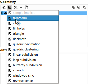
difference1)Add a filter:
 ->
-> transformEnter a value of
0.8m in theTranslate Yfield.Enter a value of
70in theRotation Zfield.
Copy the chute by pressing the
 button with the chute selected (named
transform)Enter a value of
0.8in theTranslate XfieldEnter a value of
0.6in theTranslate YfieldEnter a value of
120in theRotation Zfield
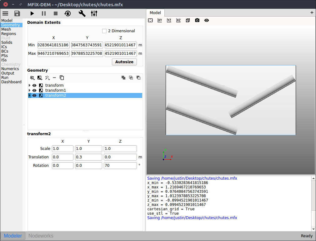
Copy the chute again by pressing the
button with the chute selected
(named transform1)Enter a value of
0.0in theTranslate XfieldEnter a value of
0.3in theTranslate YfieldEnter a value of
70in theRotation Zfield
Press the
Autosizebutton to fit the domain extents to the geometry
3.7.4. Enter the mesh
On the Mesh pane:
On the
Backgroundsub-pane
Enter
20for the x cell valueEnter
20for the y cell valueEnter
10for the z cell value
3.7.5. Create regions for initial and boundary condition specification
Select the Regions pane.
Create a region to be used for the wall boundary condition
Click the
 (all) button to create a new region
Enter a name for the region in the
Namefield (“walls”)Change the color by pressing the
ColorbuttonCheck the
Select facets (STL)checkbox
Create a region to be used as the mass inflow boundary condition
Click the
 (top) button to create a new region
Enter a name for the region in the
Namefield (“inlet”)Enter a value of
-0.4m in theFrom XfieldEnter a value of
-0.2m in theTo Xfield
3.7.6. Create a solid
On the Solids pane:
Click the
 button to create a new solid
Enter a descriptive name in the
Namefield (“glass beads”)Enter the particle diameter of
1/80m in theDiameterfieldEnter the particle density of
2500kg/m2 in theDensityfield
On the DEM sub pane:
check the
Enable automatic particle generationcheckbox and keep defaults values for all other settings.
3.7.7. Create Initial conditions
On the Initial conditions pane leave the default initial condition.
3.7.8. Create Boundary conditions
On the Boundary conditions pane:
Create a new Boundary condition by clicking the
buttonOn the
Select regiondialog, select “Mass Inflow” from theBoundary typedrop-down menuSelect the “inlet” region and click
OKOn the
glass beadssub-pane:Enter a value of
0.1in thevolume fractionfield.Enter a velocity in the
Y-axial velocityfield of-0.1m/s
Create another Boundary condition by clicking the
buttonOn the
Select regiondialog, select “No Slip Wall” from theBoundary typecombo-boxSelect the “walls” region and click
OK
3.7.9. Select output options
On the Output pane:
On the
Basicsub-pane, check theWrite VTK output files (VTU/VTP)check boxSelect the
VTKsub-paneCreate a new output by clicking the
buttonSelect
Particle Datain theOutput typecombo box.Select the “Background” region from the list to save all the cell data
Click
OKto create the outputEnter a base name for the
*.vtpfiles in theFilename basefieldChange the
Write intervalto0.1secondsSelect the
DiameterandTranslational Velocitycheck boxes.
3.7.10. Run the project
Save project by clicking
 button
Run the project by clicking the
 button
On the
Rundialog, select the default executable from the listClick the
Runbutton to actually start the simulation
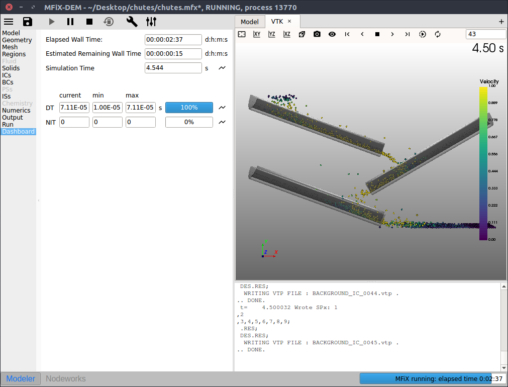
3.7.11. View results
Results can be viewed, and plotted, while the simulation is running.
Create a new visualization tab by pressing the
in the upper
right hand corner.Select an item to view, such as plotting the time step (dt) or click the
VTKbutton to view the vtk output files.