3.2. Two-dimensional fluidized bed, Two-fluid Model (TFM)¶

This tutorial shows how to create a two dimensional fluidized bed simulation using the two-fluid model. The model setup is:

Property	Value
Geometry	10 cm x 30 cm
Mesh	20 x 60
Solid diameter	200 microns (\(200 \times 10^{-6}\) m)
Solid density	2500 kg/m²
Gas velocity	0.25 m/s
Temperature	298 K
Pressure	101325 Pa

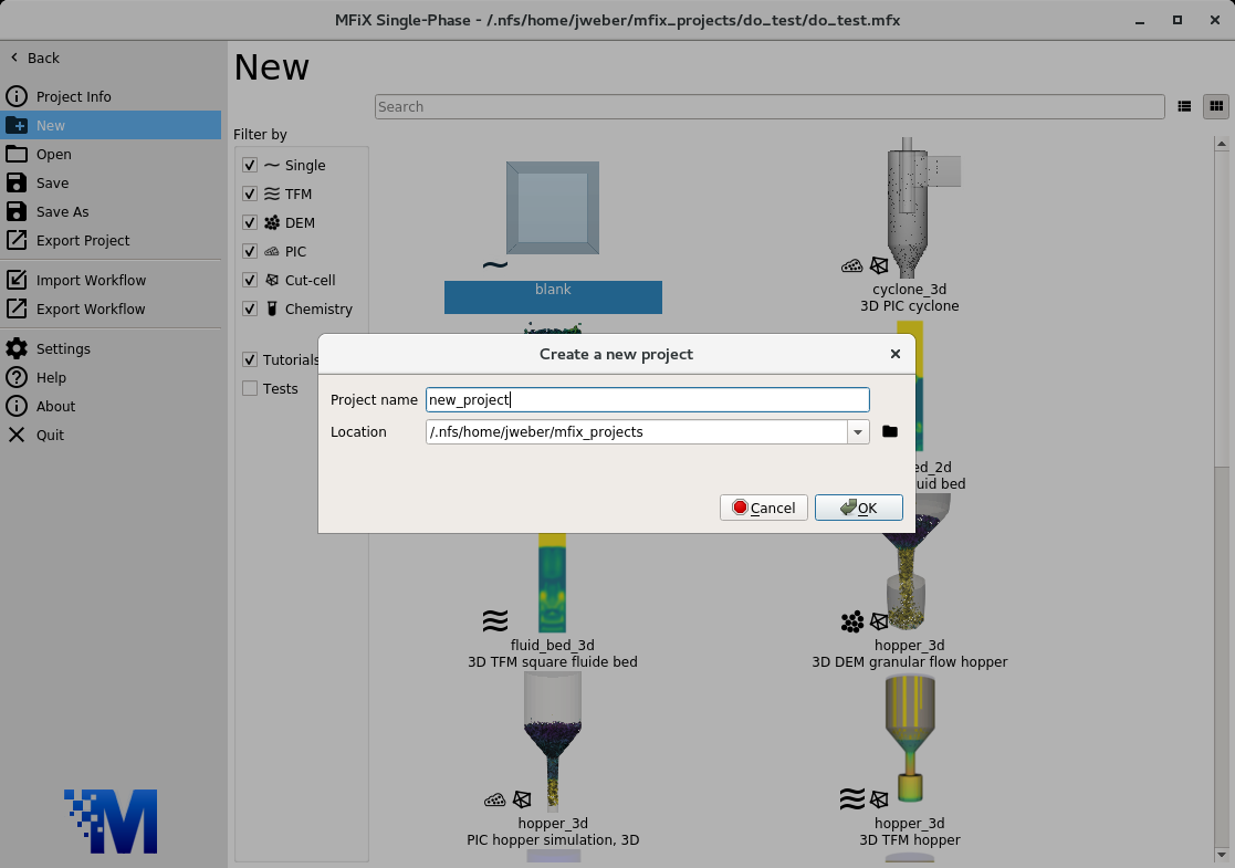
3.2.1. Create a new project¶

On the main menu select New project
Create a new project by double-clicking on “Blank” template.
Enter a project name and browse to a location for the new project.
When prompted to enable SMS workflow, answer No, we will use the standard workflow for this tutorial.

Note

A new project directory will be created in the location directory, with the name being the project name.

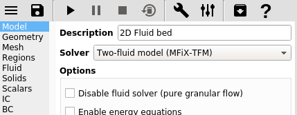
3.2.2. Select model parameters¶

On the Model pane:

Enter a descriptive text in the Description field
Select “Two-Fluid Model (MFiX-TFM)” in the Solver drop-down menu.

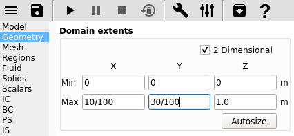
3.2.3. Enter the geometry¶

On the Geometry pane:

Select the 2 Dimensional checkbox
Enter 10/100 meters for the maximum x value
Enter 30/100 meters for the maximum y value

Note

We could have entered 0.1 and 0.3 to define the domain extents, but this example shows that simple mathematical expressions (+,-,*,/) are allowed.

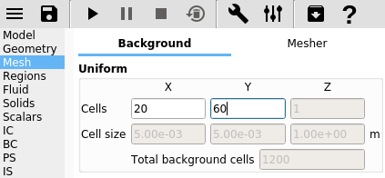
3.2.4. Enter the mesh¶

On the Mesh pane, Background sub-pane:

Enter 20 for the x cell value
Enter 60 for the y cell value

3.2.5. Create regions for initial and boundary condition specification¶

Select the Regions pane. By default, a region that covers the entire domain is already defined. This is typically used to initialize the flow field and visualize the results.

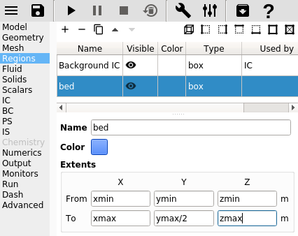
Click the (add) button to create a new region to be used for the bed initial condition.
Enter a name for the region in the Name field (“bed”)
Change the color by pressing the Color button
Enter xmin or min in the From X field
Enter xmax or max in the To X field
Enter ymin or min in the From Y field
Enter ymax/2 or max/2 in the To Y field
Enter zmin or min in the From Z field
Enter zmax or max in the To Z field

Note

Here we could have entered numerical values for the coordinates, but it is recommended to use parameters (xmin, xmax etc.) when possible. These parameters will update automatically if the “Domain Extents” change.

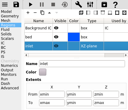
Click the (bottom) button to create a new region with the From and To fields already filled out for a region at the bottom of the domain, to be used by the gas inlet boundary condition. From Y and To Y should equal ymin, defining an XZ-plane.
Enter a name for the region in the Name field (“inlet”)

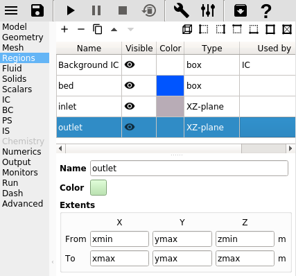
Click the (top) button to create a new region with the From and To fields already filled out for a region at the top of the domain, to be used by the pressure outlet boundary condition. From Y and To Y should equal ymax, defining an XZ-plane.
Enter a name for the region in the Name field (“outlet”)

3.2.6. Create a solid¶

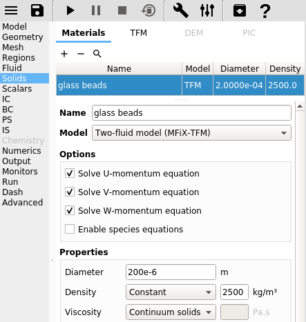
On the Solids pane:

Click the button to create a new solid
Accept the radial distribution setting (Carnahan-Starling)
Enter a descriptive name in the Name field (“glass beads”)
Keep the model as “Two-Fluid Model (MFiX-TFM)”)
Enter the particle diameter of 200e-6 m in the Diameter field
Enter the particle density of 2500 kg/m² in the Density field

3.2.7. Create Initial conditions¶

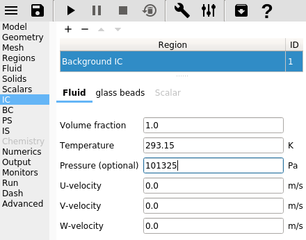
On the Initial conditions pane:

Select the already populated “Background” from the region list. This will initialize the entire flow field with air.
Enter 101325 Pa in the Pressure (optional) field

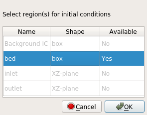
Create a new Initial Condition by pressing the button
Select the bed region created previously for the bed Initial Condition (“bed” region) and click the OK button.

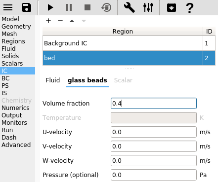
Select the solid (named previously as “glass beads”) sub-pane and enter a volume fraction of 0.4 in the Volume Fraction field. This will fill the bottom half of the domain with glass beads.

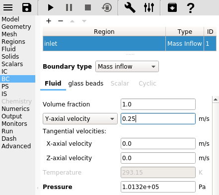
3.2.8. Create Boundary conditions¶

On the Boundary conditions pane:

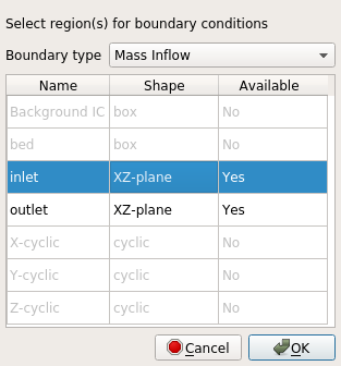
Create a new Boundary condition by clicking the button
On the Select region dialog, select “Mass Inflow” from the Boundary type drop-down menu
Select the “inlet” region and click OK

On the “Fluid” sub-pane, enter a velocity in the Y-axial velocity field of “0.25” m/s

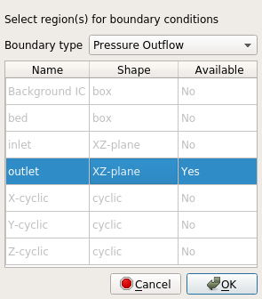
Create another Boundary condition by clicking the button
On the Select region dialog, select “Pressure outflow” from the Boundary type combo-box
Select the “outlet” region and click OK

Note

The default pressure is already set to 101325 Pa, no changes need to be made to the outlet boundary condition.

Note

By default, boundaries that are left undefined (here the left and right planes) will behave as No-Slip walls.

3.2.9. Change numeric parameters¶

On the Numerics pane, Residuals sub-pane:

Enter 0 in the Fluid Normalization field.

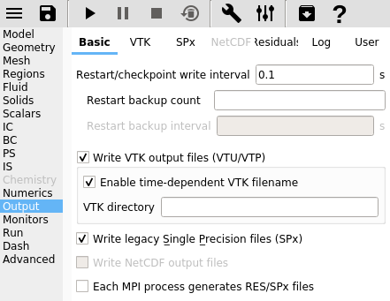
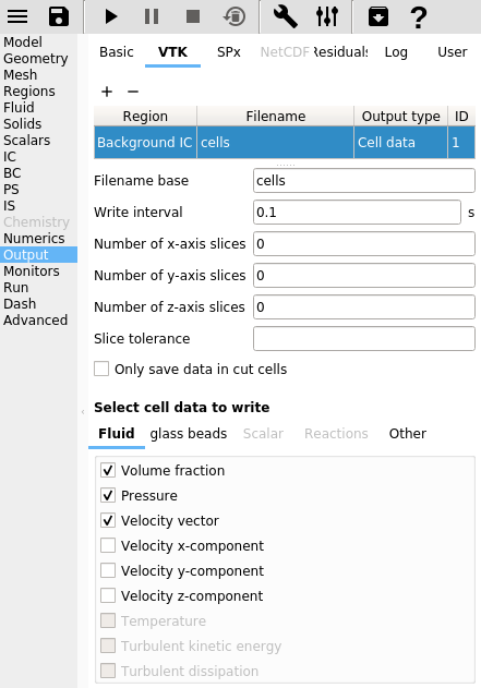
3.2.10. Select output options¶

On the Output pane:

On the Basic sub-pane, check the Write VTK output files (VTU/VTP) checkbox

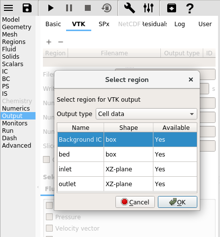
Select the VTK sub-pane
Create a new output by clicking the button
Select the “Background” region from the list to save all the cell data
Click OK to create the output

Enter a base name for the *.vtu files in the Filename base field
Change the Write interval to 0.1 seconds
Select the Volume fraction, Pressure, and Velocity vector checkboxes on the Fluid sub-sub-pane

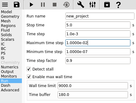
3.2.11. Change run parameters¶

On the Run pane:

Change the Time step to 1e-3 seconds
Change the Maximum time step to 1e-2 seconds

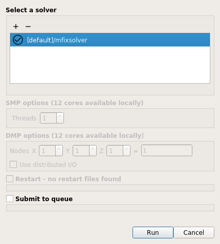
3.2.12. Run the project¶

Save project by clicking the button
Run the project by clicking the button
On the Run Solver dialog, select the executable from the combo-box
Click the Run button to actually start the simulation

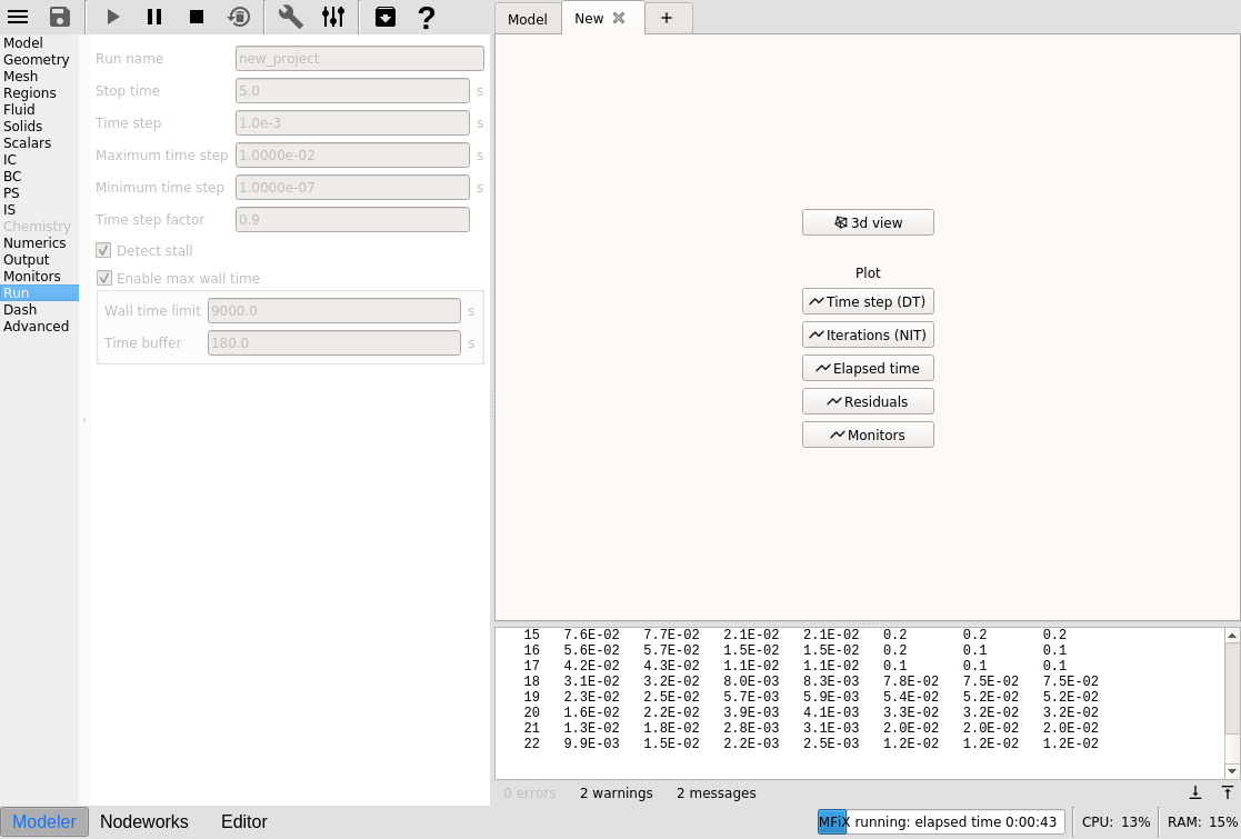
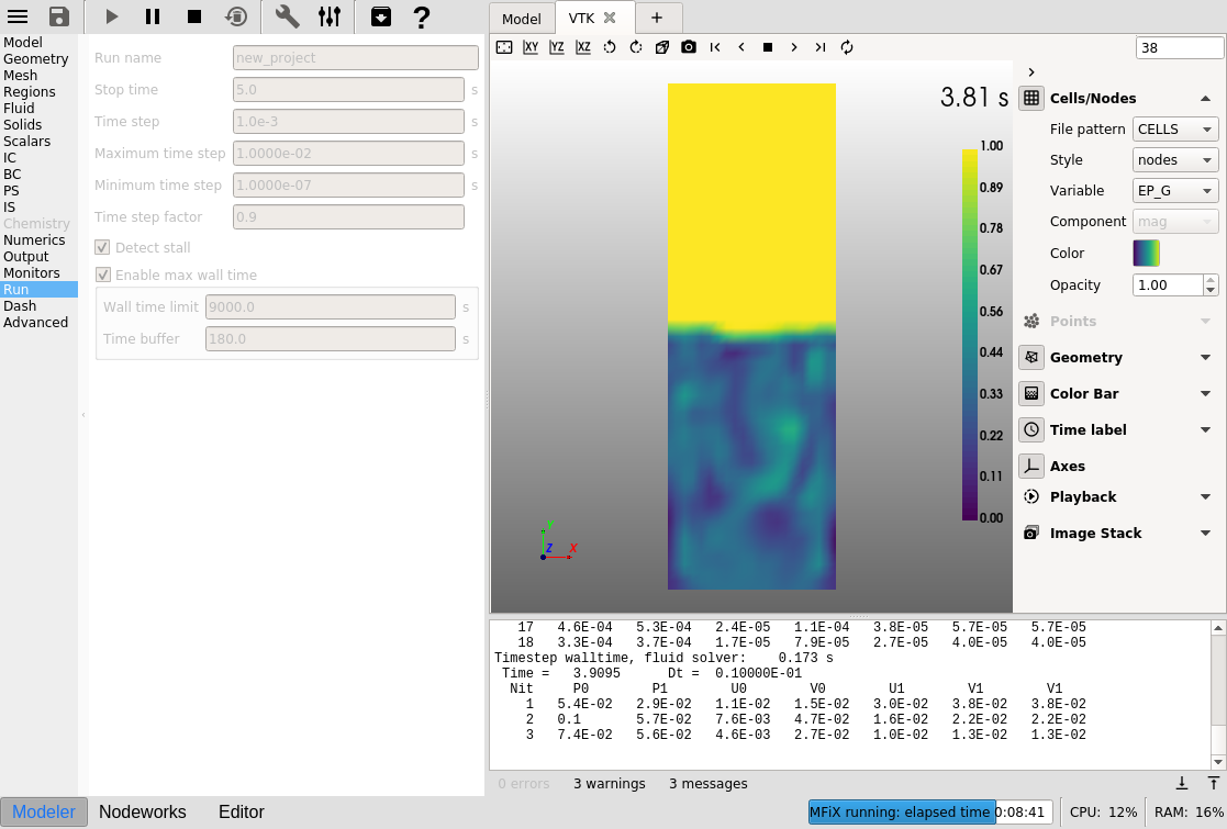
3.2.13. View results¶

Results can be viewed, and plotted, while the simulation is running.

Create a new visualization tab by pressing the next to the Model tab
Select an item to view, such as plotting the time step (dt) or click the 3D view button to view the vtk output files.

On the VTK results tab, the visibility and representation of the *.vtk files can be controlled with the menu on the side.

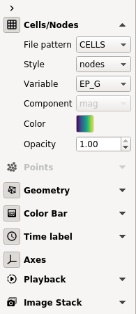
Change frames with the , , , and buttons
Click the button to play the available vtk files.
Change the playback speed under the section on the sidebar.

3.2.14. Increase grid resolution¶

For this simulation, increasing the grid resolution will better resolve the bubbles (at the expense of a slower simulation time). To do this:

Click the button and delete all simulation files.
On the Mesh pane, change the X Cells to 80 and the Y Cells to 180
On the Output pane, VTK sub-pane, change the write interval to 0.01
Save and run the project.