3.9. DEM Initial Conditions
This tutorial will illustrate various seeding options when initializing particles in an initial condition region. It is based on the 3d hopper tutorial. We will only change the initial conditions.
3.9.1. Open the 3d hopper tutorial
On the main menu, select
New projectDouble click on the “3D DEM granular flow hopper” tutorial and specify the project location.
Run the project as is to get familiar with it.
3.9.2. Change the initial condition configuration
On the
Initial conditionspane, select the “initial solids” region.Change the Solid 1 volume fraction to 0.4. Note that we are using an hexagonal lattice.
On the
Runpane, changeStop timeto 0.001. We are only interested to look at the initial conditions.Run the simulation. Visualize the particles and take a look at the output in the console and verify that seeding was successful:
Generating initial particle configuration:
Phase  1: Number of particles to seed =        18236
|-------------------------------------------------------------------|
| IC Region:   2                                                    |
|-------------------------------------------------------------------|
| Phase |   Input   |   Input   | Number of |    EPs    |   Solid   |
|   ID  | Specified |   Value   | Particles |           |   mass    |
|-------|-----------|-----------|-----------|-----------|-----------|
|    1  |   EP_S    |  4.00E-01 |     18236 |  4.00E-01 |  1.91E+02 |
|-------|-----------|-----------|-----------|-----------|-----------|
Phase  1: Successful seeding
On the
Initial conditionspane, select the “initial solids” region.Change the lattice configuration to “Cubic”.
Run the simulation. Visualize the particles and take a look at the output in the console and notice that with the cubic lattice, we are not able to reach the specified volume fraction of 0.4.
Generating initial particle configuration:
Phase  1: Number of particles to seed =        18236
|-------------------------------------------------------------------|
| IC Region:   2                                                    |
|-------------------------------------------------------------------|
| Phase |   Input   |   Input   | Number of |    EPs    |   Solid   |
|   ID  | Specified |   Value   | Particles |           |   mass    |
|-------|-----------|-----------|-----------|-----------|-----------|
|    1  |   EP_S    |  4.00E-01 |     15693 |  3.44E-01 |  1.64E+02 |
|-------|-----------|-----------|-----------|-----------|-----------|
Phase  1: Unsuccessful seeding
Instead of specifying a solids fraction, we can input a solids mass or a number of particles:
On the
Initial conditionspane, select the “initial solids” region.In the drop down menu, select “Inventory” and enter
100.0.Run the simulation and verify seeding was successful.
On the
Initial conditionspane, select the “initial solids” region.In the drop down menu, select “Particle count” and enter
10000.Run the simulation and verify seeding was successful.
The spacing between particles can also be increased:
On the
Initial conditionspane, select the “initial solids” region.Change the Solid 1 volume fraction to
0.1.Change the spacing to
0.5, run the simulation and observe how particles are more spaced out.Change the random factor to
1.0, run the simulation and observe how particles have randomly shifted from their lattice positions.
Repeat the above (spacing option) with the hexagonal lattice.
3.9.3. Particle size distribution
On the
Initial conditionspane, select the “initial solids region.Make sure the Solid 1 volume fraction is
0.1, and the lattice isHexa.Change the spacing back to
0.05, and the random factor back to1.0.In the Solids>DEM pane, Click the
 button in the Particle size distribution table (the table is initially empty if no psd have been defined yet):
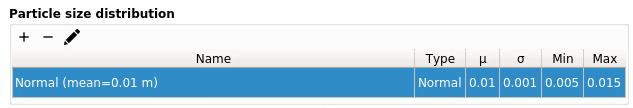
Fig. 3.1 PSD table.
Define a Normal psd:
Name:
Normal (mean = 0.01 m)(use a descriptive name).Distribution type:
NormalMean:
0.01Standard deviation:
0.001Minimum:
0.005Maximum:
0.015Plot from 0 to
0.020
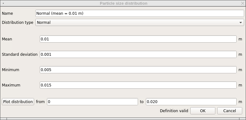
Fig. 3.2 Normal PSD definition.
Plot the psd by clicking on
Plot distribution. Verify the plot corresponds to the parameters.
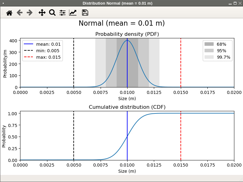
Fig. 3.3 Normal PSD plot.
Click
OK.
We now have a psd that we can use in initial or mass inlet boundary conditions.
Go to the
Initial conditionpane, go to the drop down menu under ‘Particle size distribution’ and select the psd we just defined,Normal (mean = 0.01 m).Run the simulation and visualize the particles.
Besides the Normal and Log-normal psd’s, we can also use custom distribution from a text file. It can be edited through any text editor including the GUI built-in editor. The PSD custom file is organized as follows:
The figure below shows an example of a custom PSD file. Only the first few lines are shown.
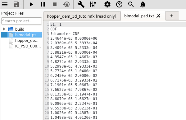
Fig. 3.4 Example of a Custom file used to define a Particle Size Distribution.
In the Solids>DEM pane, Click the
button in the Particle size distribution table, and define a custom psd:
Name:
Bimodal psd(use a descriptive name).Distribution type:
CustomSelect file: Choose
bimodal_psd.txtin the project directory.Click
Plot distribution.
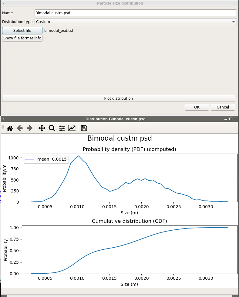
Fig. 3.5 Custom PSD.
Run the simulation and visualize particles.
Notice that we are not able to seed particles with the requested solids volume fraction of 0.1. This is because the lattice spacing is based on the largest diameter in the psd.
Change the spacing to
0.02, run the simulation and verify that we get a volume fraction of 0.1 (or near 0.1).While the simulation is running, we can visualize a histogram showing the particle size distribution. Open a new visualization viewport by clicking on the
sign on the right-most tab and select the histogram view.
This will setup a histogram plot. Users can change the file to view, the variable, number of bins and style
(lines or bars). To adjust the scale, right-click on the view and enter the axis limits or have them
be automatically updated based on data.
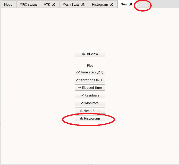
Fig. 3.6 Opening a histogram view.
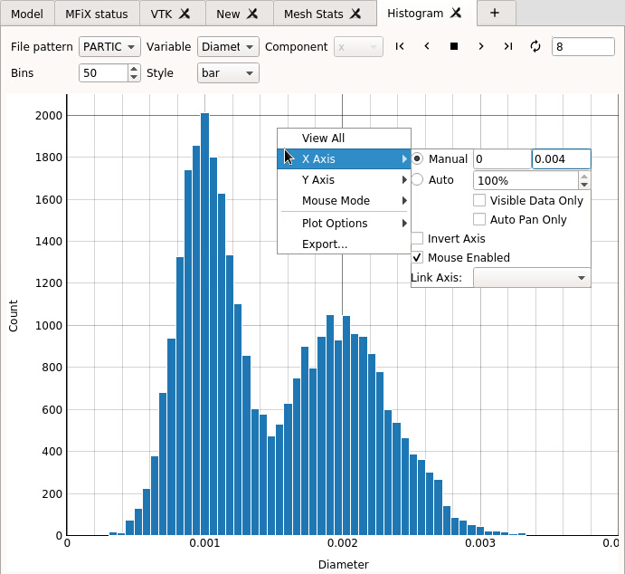
Fig. 3.7 Visualizing particle diameter histogram.
3.9.4. Reading initial particle data from a text file
We can read the initial particle data from a text file, called particle_input.dat.
The format of this file has changed in the 20.3 release. The old file version can still
be used but it is recommended to use the latest format.
The new format allows to either read variables or set a constant value for all particles. The file contains a long header where information about the data is specified. This controls how many columns and which variables are read from the file. Next, the data section contains the data for each particle. Each column corresponds to a variable. In 3D, the first 3 columns are always the x,y and z coordinates of the particle’s center. In 2D, the first 2 columns are always the x and y coordinates of the particle’s center. There are two options for the other variables: either read the data for each particle in the next column, or assign a constant value to all particles.
Below is an example of a particle_input.dat file (the line number is shown on the left and it
not part of the data itself):
Line 1 : File version. Do not change this line.
Lines 2-18 : Instructions to use the file.
Line 19 : This is a 3D geometry. The first 3 columns in the data section will be x,y,z.
Line 20 : We will read data for 35361 particles.
Line 24 : We always read coordinates in the first 2 or 3 columns (do not change)
Line 25 : We do not read particle’s phase ID for each particle. It is assigned a constant value: 1
Line 26 : We will read the particle’s diameter in the next column (column#4).
Line 27 : We do not read particle’s density. It is assigned a constant value: 2500.0 kg/m^3
Line 25 : We do not read particle’s velocity. It is assigned a constant value: (u,v,w) = (0.0,0.0,0.0) m/s
Lines 29-30: This is a cold, non reacting case, we do not read Temperature or species.
Line 31 : We do not have user scalars, so we do not read them.
Lines 32-34: Data header
The data starts on Line 35. Based on the above settings, we need to read, x,y,z, and the diameter of each particles, i.e., 4 columns, for 35361 particles. Only the first few lines of the data is shown.
1 Version 2.0
2 ========================================================================
3 Instructions:
4 Dimension: Enter "2" for 2D, "3" for 3D (Integer)
5 Particles: Number of particles to read from this file (Integer)
6 For each variable, enter whether it will be read from the file
7 ("T" to be read (True), "F" to not be read (False)). When not read, enter the
8 default values assign to all particles.
9 Coordinates are always read (X,Y in 2D, X,Y,Z in 3D)
10 Phase_ID, Diameter, Density, Temperature are scalars
11 Velocity requires U,V in 2D, U,V,W in 3D
12 Temperature is only read/set if the energy equation is solved
13 Species are only read/set if the species equations are solved, and requires
14 all species to be set (if phase 1 has 2 species and phase 2 has 4 species,
15 all particles must have 4 entries, even phase 1 particles (pad list with zeros)
16 User scalars need DES_USR_VAR_SIZE values
17 Data starts at line 35. Each column correspond to a variable.
18 ========================================================================
19 Dimension:    3
20 Particles:    35361
21 ========================================================================
22 Variable      Read(T/F)     Default value (when Read=F)
23 ========================================================================
24 Coordinates:     T          Must always be T
25 Phase_ID:        F          1
26 Diameter:        T
27 Density:         F          2500.0
28 Velocity:        F          0.0 0.0 0.0
29 Temperature:     T          (Ignored if energy eq. is not solved)
30 Species:         T          (Ignored if species eq. are not solved)
31 User_Scalar:     T          (Ignored if no user scalars are defined)
32 ========================================================================
33     X (m)           Y (m)           Z (m)       Diameter (m)
34 ========================================================================
35 -5.07749E-02    -7.98147E-01    -2.00612E-01    9.71052E-03
36 -4.86164E-02    -8.16202E-01    -2.25035E-01    8.34185E-03
37 -3.16460E-02    -8.13702E-01    -2.19164E-01    1.09747E-02
38 -3.32833E-02    -8.25178E-01    -2.19393E-01    9.67983E-03
39 -2.48844E-02    -8.30159E-01    -2.16423E-01    9.84182E-03
40 -8.57591E-03    -8.38121E-01    -2.08773E-01    9.92759E-03
41 -2.75312E-03    -8.32665E-01    -2.00770E-01    1.07560E-02
42 1.57276E-02     -8.37839E-01    -2.08196E-01    1.04387E-02
43 1.96605E-02     -8.31447E-01    -2.15105E-01    9.97808E-03
44 2.71083E-02     -8.26450E-01    -2.19492E-01    9.99619E-03
45 3.55440E-02     -8.28885E-01    -2.15687E-01    9.15771E-03
46 4.45244E-02     -8.28239E-01    -2.11771E-01    1.05089E-02
47 4.70488E-02     -8.22092E-01    -2.19129E-01    9.33350E-03
This data files contains particles that have settled in the top half of the hopper. To use it as initial conditions:
In the Solids>DEM pane, uncheck
Enable automatic particle generation, and enter a data file particle count of35361. An entry is required to maintain compatibility with the old format, but the value on line 20 of the version 2.0 file will actually be used.In the
Initial conditionpane, delete theInitial solidsinitial condition.In the
Runpane, set the stop time to 1.0 seconds.Run the simulation. You should see the initial configuration shown below:
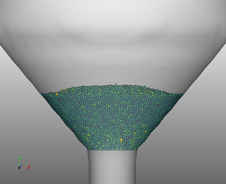
Fig. 3.8 Example of a DEM initial condition using particle_input.dat version 2.0.