Ex. 2: Optimization
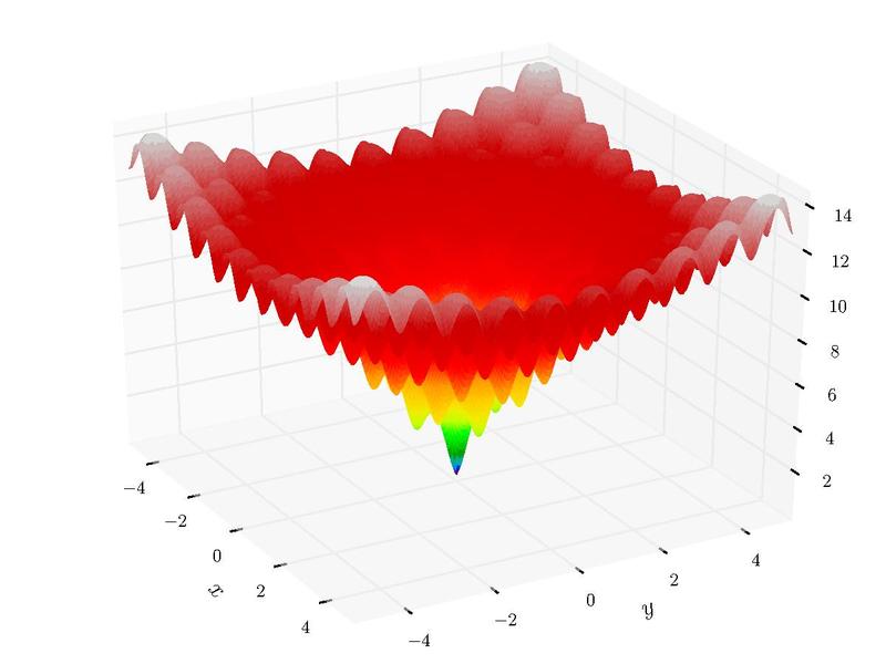
This example demonstrates the optimization of the Ackley function, which is commonly used to test the performance of optimization algorithms. The function has many local minima and one global minimum at \(f(0,0)=0\).
Populate the Nodes
The Node Wizard conveniently provides functionality to populate all the nodes and provides a collection of optimization test functions, including the Ackley function. To construct the workflow quickly and focus on the optimization aspect, use the wizard by:
Click on the
button to launch the wizard.
Click on the
Optimizationtab and set theFunction to be optimizedtoAckleyand level theMethodassurrogate.Click
Populate Nodes
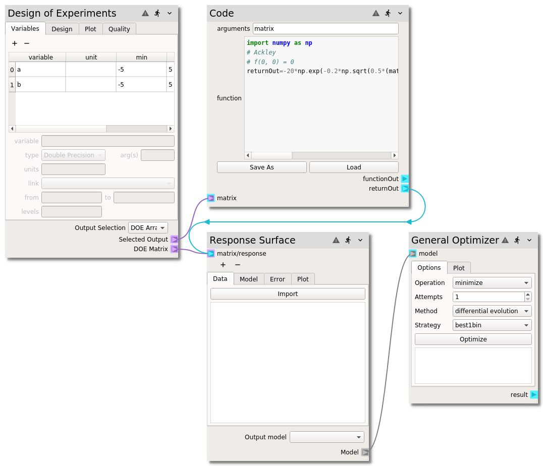
You should now have a collection of nodes including:
a Design of Experiments node with two variables, using the hammersly method with 1000 samples
a
Codenode with the Ackley functiona Response Surface node with the
radial basis functionselected, anda General Optimizer node
that looks like this:
Local Optimization
To demonstrate the challenge with black-box optimization, we will first try using a local minimization method:
On the General Optimizer, change the number of attempts to
10.Select
localfrom theMethodcombo-box. TheLocal Methodcombo-box should appear with theNelder-Meadmethod selected.Run all the nodes by pressing
 button on the application toolbar.
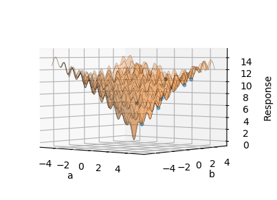
After all the nodes have been run, the results of the 10 minimization attempts are displayed. Notice how each of the 10 attempts seems to provide a different “optimum”. This happens because each attempt has an initial condition which is randomly picked from inside the ranges of the variables specified in the Design of Experiments node. This local minimization method frequently gets stuck in the many local minima of the Ackley function.
The attempts can be visualized on the Plot tab of the General Optimizer
node, where the surface is the sampled function and the dots are the
optimization attempts. Note how these particular attempts never found the global
minimum:
Global Optimization
Global optimization routines try to avoid getting stuck in local minima. One method provided in the General Optimizer node that works well is Differential Evolution.
To use this method:
select
differential evolutionfrom theMethodcombo-boxpress the
Optimizebutton on the General Optimizer node
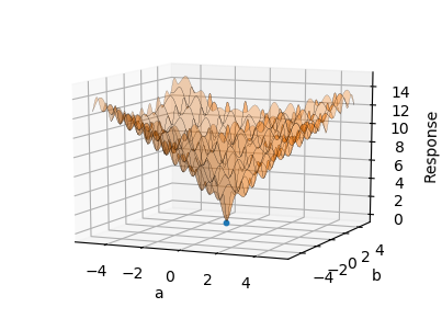
After the node has run, all 10 optimization attempts should be roughly the same value, \(f(-0.02, -0.02)=0.19\). The differential evolution algorithm did a good job of avoiding the local minimas and finding the true minimum. Unfortunately, this value is not precisely the true minimum, which should be \(f(0,0)=0\). The problem is that there are not enough samples at or around the true minimum for the surrogate model, constructed in the Response Surface, to accurately represent the sharp minimum of the Ackley function.
Response Surface Refinement
After an optimum has been found, the response surface can be refined around that optimum to get closer to the true optimum. In this particular case, lets see if we can get closer to the mathematical optimum. To do this, we will leave the original samples in-place and add new samples around the optimum:
Duplicate the Design of Experiments node and
Codenode bySelecting the Design of Experiments node by clicking on the title.
While holding
Ctrlon the keyboard, select theCodenode by clicking on its title.Copy the selected nodes by either pressing
Ctrl+con the keyboard orright-clickand selectCopyfrom the menu.left-clickto the left of the Response Surface node.Paste the nodes by pressing
Ctrl+von the keyboard orright-clickand selectPastefrom the menu.
Add a
Matrix/Responseterminal to the Response Surface node by pressing the button below the existing
 Matrix/Responseterminal.Connect the terminals of the copied nodes by
Connecting the
Selected Outputterminal of the copied Design of Experiments node to thematrixterminal of the copiedCodenode.Connecting the
returnOutterminals of the copiedCodenode to the newMatrix/Response 1terminal of the Response Surface node.Connecting the
DOE Matrixterminal of the copied Design of Experiments node to the newMatrix/Response 1terminal of the Response Surface node.
Adjust the variable ranges of the copied Design of Experiments node by
Select the
variabletabSelect variable
aand changed thefromvalue to-0.1and thetovalue to0.1.Select variable
band changed thefromvalue to-0.1and thetovalue to0.1.On the
Designtab, change the number ofSamplesto100.On the
Designtab, press theBuildbutton to build the samples.
Adjust the response surface in the Response Surface node node by
Select the
ModeltabSelect the
radial basis functionfrom the table.Change the
Functionfrommultiquadrictocubic
Run all the nodes by pressing
button on the application toolbar.
By adding the additional samples, the found optimum (\(f(-0.0007, 0.001)=0.02\)) is closer to the analytic solution (\(f(0,0)=0\)). You should have a workflow that looks like this:

Note
See how close you can get to the true solution of \(f(0,0)=0\) by changing the samples and response surface model settings.