Poly Projection

Overview

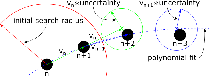
Poly projection is a projection based approach to finding the same object across successive frames. By fitting the past particle locations with a polynomial, the polynomial can be evaluated to predict where the particle location should be. The closest particle to the projected location is then used. The algorithm is:

Frame	Description of step
n	An object is found
n+1	Using the default search radius $r_{default}$, find the closest point to the previous location, $p(n)$.
n+2	Using the previous two points ($p(n)$ and $p(n+1)$), calculate the velocity, $v(n)$. Using this velocity, project the next location, $p_{predict}(n+2)=p(n)\ast v(n)$. Finally, find the closest object to the predicted location, within the search radius, $r_{search}$.
n+3	Using the previous three points ($p(n)$, $p(n+1)$, and $p(n+2)$), fit a polynomial, $f()$. Evaluate the polynomial at the current frame to predict the object location, $p_{predict}(n+3)=f(n+3)$. Finally, find the closest object to $p_{predict}(n+3)$, within the search radius, $r_{search}$.
n+i	Repeat the n+3 step, using some or all the previous points to fit a new polynomial, until an object can not be found within the search radius at the projected location, $p_{predict}(n+i)=f(n+i)$

Where the following variables are defined as:

Variable	Description
$p(n)$	x, y, z position of the object
$f(n)$	polynomial fit to some or all of the previous positions
$v(n)$	velocity of the object
$uncertainty$	multiplier to calculate search radius
$r_{minimum}$	minimum search radius
$r_{search}(n)$	search radius, $max(uncertainty\ast v(n-1),r_{minimum})$

Graphically, the algorithm looks like:

Limitations

For a given search area, there can potentially be many objects. The current implementation defaults to the closest object to the $p_{predict}(n)$. Depending on the speed of the objects, the closest object might not be the same object, especially on the first step while using the default search area. One way to overcome this issue is to use a sufficiently high sample rate (frame rate) such that the displacement of the object is less than the center of its closest neighbor.

The other method (not implemented yet) is to try matching objects using either the intensity or a group of pixels (tile). This can be used to match objects as opposed to picking the closest object.

Polynomial Order

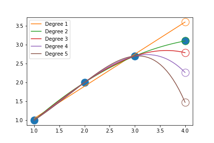
For most applications, a polynomial degree of 2 should be sufficient to capture and predict the motion of objects with acceleration. A polynomial with a degree of 2 represents the following kinematic equation:

$$d=vt+\frac{1}{2}a{t}^2$$

where $d$ is the displacement, $v$ is the velocity, $t$ is time and $a$ is acceleration. High order polynomials can also have wild oscillations, causing predictions to be inaccurate as depicted below:

In practice, it has been observed that higher order polynomials can capture collisions better then second order polynomials. Sample rates also need to be sufficiently high to capture multiple points during the collision as well.

Neighbor Search

A KDTree, implemented in scipy, is constructed from the objects of each frame. This tree is then used to find neighboring objects to a given point ($p_{predict}(n)$).