4.2. DEM02: Bouncing particle
This case provides a comparison between the MFIX-DEM linear spring-dashpot collision model and the hard sphere model where collisions are instantaneous. The hard sphere model can be seen as the limiting case where the normal spring coefficient is large, \(k_{n} \rightarrow \infty\). This case was originally reported in [8].
4.2.1. Description
A smooth (frictionless), spherical particle falls freely under gravity from an initial height, \(h_{0}\), and bounces upon collision with a fixed wall Fig. 4.1. Assuming that the collision is instantaneous, the maximum height the particle reaches after the first collision (bounce), \(h_{1}^{\mathrm{\max}}\), is given by
where \(r_{p}\) is the particle radius, and \(e_{n}\) is the restitution coefficient. A general expression for the maximum height following the \(k^{\text{th}}\) bounce is
4.2.2. Setup
Computational/Physical model |
|||
|---|---|---|---|
1D, Transient |
|||
Granular flow (no gas) |
|||
Gravity |
|||
Thermal energy equation is not solved |
|||
Geometry |
|||
Coordinate system |
Cartesian |
||
x-length |
1.0 |
(m) |
|
y-length |
1.0 |
(m) |
|
z-length |
1.0 |
(m) |
|
Solids Properties |
|||
Normal spring coefficient, \(k_{n}\) |
varied |
(N·m-1) |
|
Restitution coefficient, \(e_{n}\) |
varied |
( ) |
|
Friction coefficient, \(\mu\) |
0.0 |
( ) |
|
Solids 1 Type |
DEM |
||
Diameter, \(d_{p}\) |
0.2 |
(m) |
|
Density, \(\rho_{s}\) |
2600 |
(kg·m-3) |
|
Boundary Conditions |
|||
All boundaries |
Solid walls |
4.2.3. Results
Simulations of a freely-falling particle dropped from an initial height of 0.5m were conducted for three normal spring coefficients, \(\lbrack 0.5,\ 5.0,\ 50.0\rbrack \times 10^{5}\) N·m-1, and six restitution coefficients, [0.5, 0.6, 0.7, 0.8, 0.9, 1.0]. All simulations employed the Adams-Bashforth time-stepping method. The maximum height attained after the kth collision for all cases is shown in Fig. 4.5.
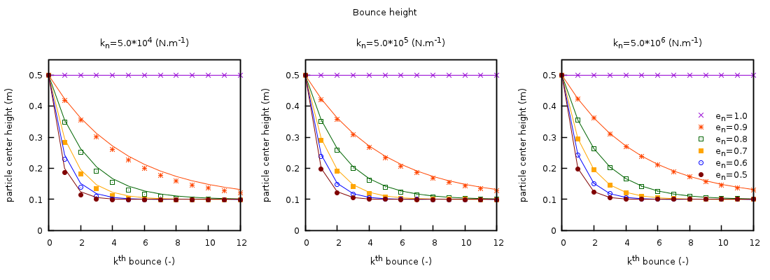
Fig. 4.5 Comparison between the analytic solution from a hard-sphere model (solid lines) and MFIX-DEM (symbols) of the maximum height reached after the kth wall collision for a freely falling particle. Three values for the normal spring coefficient are used (left to right) with six restitution coefficients.
Fig. 4.6 illustrates the percent relative difference between the analytical solution for a hard-sphere model and the MFIX-DEM simulation. In the limit of the hard-sphere model (shown left to right by an increasing spring coefficient), the difference between the two collision models decreases.
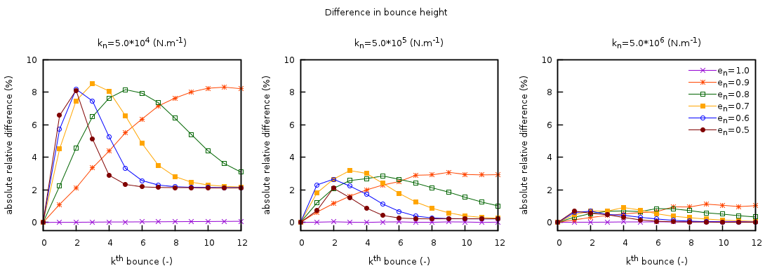
Fig. 4.6 Percent relative difference between the analytic solution for a hard-sphere model and MFIX-DEM of the maximum height reached after the kth wall collision for a freely falling particle. Three values for the normal spring coefficient are used (left to right) with six restitution coefficients.