5.3. PIC03: Advection in time varying flow field – parcel volume deposition
5.3.1. Description
In this case the arrangement of 480 parcels having a radius of 0.15 m centered at the origin is considered. The objective is to test the following:
Periodic boundaries
Parcel volume deposition on Eulerian cells
The time varying flow-field is prescribed using Eq.5.3, where the time period T is 0.25 seconds. The domain under consideration and its discretization are identical to the set-up described in Section 2.2.1. The initial parcel configuration is specified through a particle_input.dat file.
5.3.2. Setup
Computational/Physical model |
|||
|---|---|---|---|
3D, Transient |
|||
Multiphase |
|||
Gravity |
|||
Thermal energy equation is not solved |
|||
Turbulence equations are not solved (Laminar) |
|||
Uniform mesh |
|||
First order upqind discritization scheme |
|||
Geometry |
|||
Coordinate system |
Cartesian |
Grid partitions |
|
x-length |
1.0 |
(m) |
32 |
y-length |
1.0 |
(m) |
32 |
z-length |
1.0 |
(m) |
32 |
Material |
|||
Gas density, \(\rho_{g}\) |
1.2 |
(kg·m-3) |
|
Gas viscosity, \(\mu_{g}\) |
1.8E-05 |
(Pa·s) |
|
Solids Type |
PIC |
||
Diameter, \(d_{p}\) |
0.01 |
(m) |
|
Density, \(\rho_{s}\) |
2700 |
(kg·m-3) |
|
Solids Properties (PIC) |
|||
Pressure linear scale factor, \(P_{s}\) |
100.0 |
(Pa) |
|
Exponential scale factor, \(\gamma\) |
3.0 |
(-) |
|
Statistical weight |
1 |
(-) |
|
Initial Conditions |
|||
x-velocity, \(u_{g}\) |
(m·s-1) |
||
y-velocity, \(v_{g}\) |
(m·s-1) |
||
z-velocity, \(w_{g}\) |
(m·s-1) |
||
Gas volume fraction, \(\epsilon_{g}\) |
1.0 |
(-) |
|
Gas volume fraction at packing, \(\epsilon_{g}^{*}\) |
0.4 |
(-) |
|
Pressure, \(P_{g}\) |
101,325 |
(Pa) |
|
Boundary Conditions |
|||
All boundaries are cyclic |
A value of 0.25 is chosen for the time period T and the simulations are run for a total duration of 4 seconds which is equivalent to 16 cycles. The initial parcel configuration and velocities are specified through a particle_input.dat file, typical of MFiX runs that require an exact particle arrangement.
5.3.3. Results
Once the simulation begins, parcels move in all possible directions and across the periodic boundaries as shown in Fig. 5.3. The volume conservation is examined by comparing the volume fractions of fluid and solid during the simulation as given in Table 5.6. The volume fraction of fluid is calculated by the code, based on interpolation of solid volumes on to the Eulerian cells and the volume fraction of solids is calculated using the particle count. It can be seen that fluid and solid volume fractions (\(\epsilon_{g},\epsilon_{s}\)) do sum to 1 (very close to machine precision). This is indicated by the negligible relative error of the sum of phasic volume fractions in Table 5.6. Hence, this study concluded that the implementation of routines pertaining to periodicity and parcel-fluid interpolation are verified.
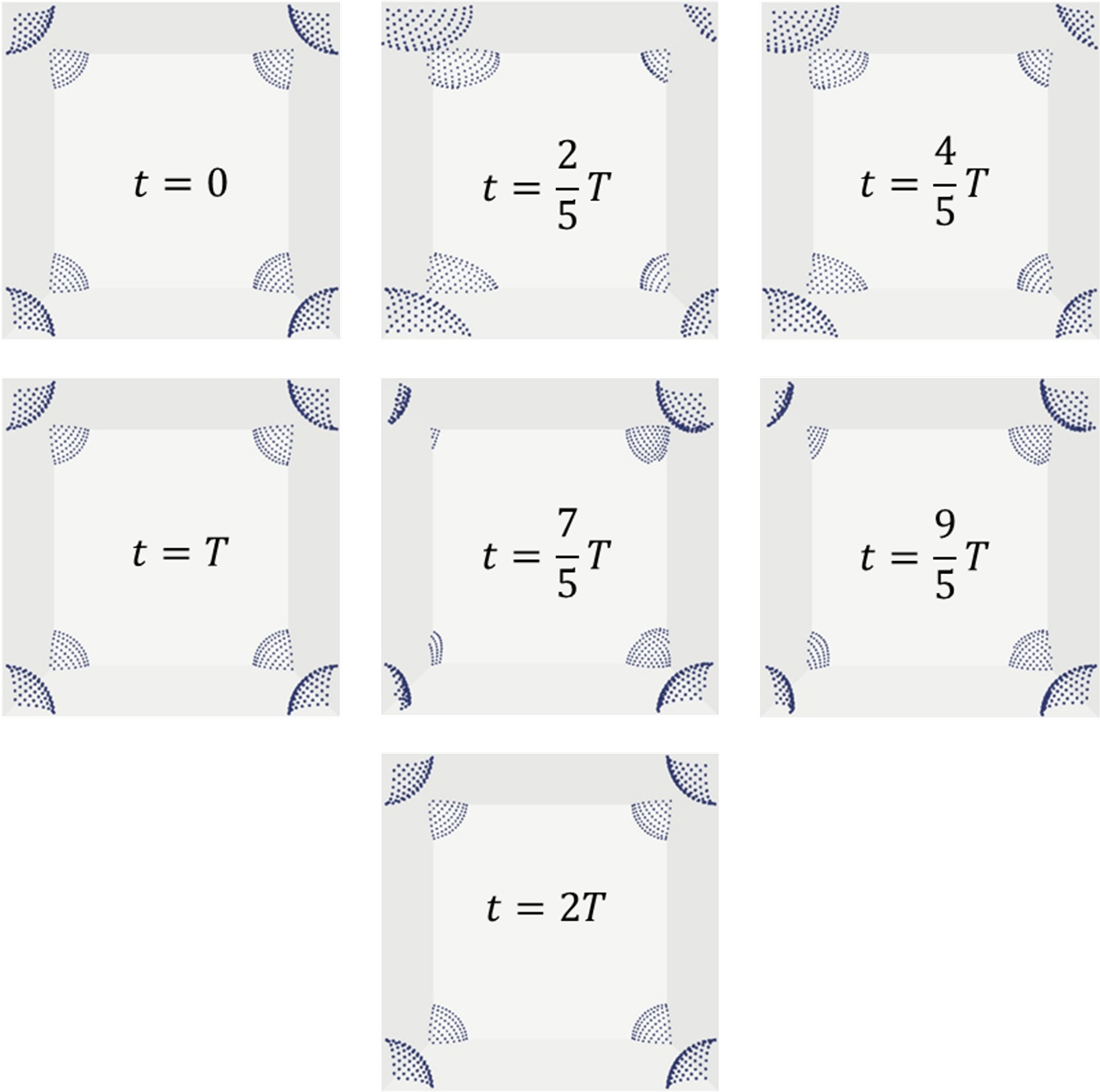
Fig. 5.3 Instantaneous location of parcels for the configuration centered at X=0 m, Y=0 m, Z=0 m. Time stamps are provided inside each snapshot.
Physical Time (s) |
Cycle |
\(\epsilon_{s}\) |
\(\epsilon_{g}\) |
Absolute Error |
0.25 |
1 |
2.51E-04 |
9.997487E-01 |
6.66E-16 |
0.50 |
2 |
2.51E-04 |
9.997487E-01 |
8.88E-16 |
0.75 |
3 |
2.51E-04 |
9.997487E-01 |
3.33E-16 |
1.00 |
4 |
2.51E-04 |
9.997487E-01 |
8.88E-16 |
1.25 |
5 |
2.51E-04 |
9.997487E-01 |
4.44E-16 |
1.50 |
6 |
2.51E-04 |
9.997487E-01 |
1.33E-15 |
1.75 |
7 |
2.51E-04 |
9.997487E-01 |
8.88E-16 |
2.00 |
8 |
2.51E-04 |
9.997487E-01 |
0 |
2.25 |
9 |
2.51E-04 |
9.997487E-01 |
1.67E-15 |
2.50 |
10 |
2.51E-04 |
9.997487E-01 |
4.44E-16 |
2.75 |
11 |
2.51E-04 |
9.997487E-01 |
2.22E-16 |
3.00 |
12 |
2.51E-04 |
9.997487E-01 |
0 |
3.25 |
13 |
2.51E-04 |
9.997487E-01 |
4.44E-16 |
3.50 |
14 |
2.51E-04 |
9.997487E-01 |
1.11E-15 |
3.75 |
15 |
2.51E-04 |
9.997487E-01 |
1.11E-15 |
4.00 |
16 |
2.51E-04 |
9.997487E-01 |
6.66E-16 |