5.5. PIC05: Evaporation
5.5.1. Description
This case is used to verify the transport equations governing energy and species conservation. The setup consists of a single parcel representing a droplet suspended in a humidified air stream. This reflects the wet bulb phenomenon, where evaporation from the droplet results in a lowered humidified air temperature. The following reaction represents species transfer from the suspended droplet:
Fifteen seconds of physical time is simulated to ensure the droplet achieves a steady-state (SS) temperature. The SS temperature should then compare with the theoretical wet-bulb temperature.
5.5.2. Setup
Computational/Physical model |
|||
|---|---|---|---|
3D, Transient |
|||
Multiphase |
|||
Gravity |
|||
Turbulence equations are not solved |
|||
Uniform mesh |
|||
First order upqind discritization scheme |
|||
Geometry |
|||
Coordinate system |
Cartesian |
Grid partitions |
|
x-length |
0.01 |
(m) |
1 |
y-length |
0.01 |
(m) |
1 |
z-length |
0.01 |
(m) |
1 |
Material |
|||
Gas density, \(\rho_{g}\) |
Ideal gas law |
(kg·m-3) |
|
Solids Type |
PIC,DEM |
||
Diameter, \(d_{p}\) |
0.2 |
(mm) |
|
Density, \(\rho_{s}\) |
958.6 |
(kg·m-3) |
|
Solids Properties (PIC) |
|||
Pressure linear scale factor, \(P_{s}\) |
0.0 |
(Pa) |
|
Exponential scale factor, \(\gamma\) |
1.0 |
(-) |
|
Statistical weight |
25 |
(-) |
|
Solids Properties (DEM) |
|||
Coefficient of friction, \(\mu_{pp},\mu_{pw}\) |
0.0 |
(-) |
|
Coefficient of restitution, \(e_{pp},e_{pw}\) |
1.0 |
(-) |
|
Spring constant, \(k_{pp},k_{pw}\) |
0.1 |
(kg·m-1) |
|
Initial Conditions |
|||
x-velocity, \(u_{g}\) |
3.0 |
(m·s-1) |
|
y-velocity, \(v_{g}\) |
0.0 |
(m·s-1) |
|
z-velocity, \(w_{g}\) |
0.0 |
(m·s-1) |
|
Gas volume fraction, \(\epsilon_{g}\) |
0.999894 |
(-) |
|
Gas volume fraction at packing, \(\epsilon_{g}^{*}\) |
0.4 |
(-) |
|
Pressure, \(P_{g}\) |
101,325 |
(Pa) |
|
Gas temperature, \(T_{g}\) |
303.15 |
(K) |
|
Solid temperature, \(T_{s}\) |
303.15 |
(K) |
|
Species fraction of air, \(X_{g1}\) |
Varied |
(-) |
|
Species fraction of water vapor, \(X_{g2}\) |
Varied |
(-) |
|
Boundary Conditions |
|||
West boundary |
\(u_{g}\) Varied |
(kg·s-1) |
Mass inflow |
\(X_{g1},X_{g2}\) Varied |
(-) |
||
East boundary |
101,325 |
(Pa) |
Pressure outflow |
North and South boundaries |
Free-slip walls |
||
Top and Bottom boundaries |
Free-slip walls |
5.5.3. Results
MFiX-PIC and MFiX-DEM simulations are performed by varying the relative humidity of surrounding air. Table 5.8 summarizes the different settings of relative humidity and the corresponding wet bulb temperatures. Based on the comparison of the data from [17] it can be concluded that the predictions from MFiX-PIC simulations are accurate Table 5.8. Also, the results are consistent with the predictions from MFiX-DEM.
Rel. Humidity (%) |
\(X_{g1}\) |
\(X_{g2}\) |
Mass Flow Rate (g/s) |
Wet Bulb T (°C) |
0 |
1.000000 |
0.000000 |
0.349315 |
10.5 |
10 |
0.997390 |
0.002610 |
0.348762 |
13.2 |
20 |
0.994771 |
0.005229 |
0.348208 |
15.7 |
30 |
0.992144 |
0.007856 |
0.347655 |
18.0 |
40 |
0.989509 |
0.010491 |
0.347102 |
20.1 |
50 |
0.986865 |
0.013135 |
0.346548 |
22.0 |
60 |
0.984212 |
0.015788 |
0.345995 |
23.8 |
70 |
0.981552 |
0.018448 |
0.345442 |
25.5 |
80 |
0.978882 |
0.021118 |
0.344888 |
27.1 |
90 |
0.976204 |
0.023796 |
0.344335 |
28.6 |
100 |
0.973518 |
0.026482 |
0.343281 |
30.0 |
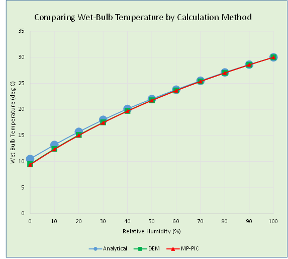
Fig. 5.6 Comparison of wet bulb temperatures between data, MFiX-DEM and MFiX-PIC.