5.4. PIC04: Particle-Settling in Fluid

5.4.1. Description

MFiX-TFM, MFiX-DEM and MFiX-PIC are used to simulate the problem of particle settling. Spatial locations of concentration fronts at time t = 1 seconds are compared with the analytical expression given by,

(5.4)\[x(t) = x_{0} + t u_{shock}\]

The velocity of propagation of the shock wave (derived in Appendix B) is given by,

(5.5)\[u_{shock} = - \Bigg( j + \frac{\big(\epsilon_{s} \epsilon_{g} u_{r}\big)_{B} - \big(\epsilon_{s} \epsilon_{g} u_{r}\big)_{A}}{\epsilon_{sB} - \epsilon_{sA}} \Bigg)\]

where the subscripts A and B denote the regions on either side of the shock as shown in Fig. 7.2. The volumetric flux is 0 in the case of settling. Also, the particle volume fraction in region A is 0 for the shock front traveling downwards. Hence the location of the shock is given by,

(5.6)\[x(t) = x_{0} -t\big(\epsilon_{g0} u_{r0}\big)\]

where, \(\epsilon_{g0}\) is the initial gas volume fraction. The relative velocity using the Stokes drag law is given by,

(5.7)\[u_{r0} = \frac{g \Delta \rho d_{p}^{2}}{18 \mu_{g}}\epsilon_{g0}^{3.65}\]

The location of the shock front corresponding to filling is given by,

(5.8)\[x(t) = -t \Bigg( \frac{\big(\epsilon_{s}^{*} \epsilon_{g}^{*} u_{r}^{*}\big) - \big(\epsilon_{s0} \epsilon_{g0} u_{r0}\big)_{A}}{\epsilon_{s}^{*} - \epsilon_{s0}} \Bigg)\]

5.4.2. Setup

Table 5.7 PIC-04 Setup, Initial and Boundary Conditions.

Computational/Physical model
3D, Transient
Multiphase
Gravity
Thermal energy equation is not solved
Turbulence equations are not solved (Laminar)
Uniform mesh
First order upqind discritization scheme
Geometry
Coordinate system	Cartesian		Grid partitions
x-length	0.02	(m)	5
y-length	1.0	(m)	100
z-length	0.02	(m)	5
Material
Gas density, \(\rho_{g}\)	1000.0	(kg·m-3)
Gas viscosity, \(\mu_{g}\)	0.001	(Pa·s)
Solids Type	PIC,DEM,TFM
Diameter, \(d_{p}\)	0.01	(m)
Density, \(\rho_{s}\)	2700	(kg·m-3)
Solids Properties (PIC)
Pressure linear scale factor, \(P_{s}\)	10.0	(Pa)
Exponential scale factor, \(\gamma\)	3.0	(-)
Statistical weight	5	(-)
Solids slip velocity factor	0.5	(-)
Solids Properties (DEM)
Coefficient of friction, \(\mu_{pp},\mu_{pw}\)	0.1	(-)
Coefficient of restitution, \(e_{pp},e_{pw}\)	0.9	(-)
Spring constant, \(k_{pp},k_{pw}\)	100.0	(kg·m-1)
Initial Conditions
x-velocity, \(u_{g}\)	0.0	(m·s-1)
y-velocity, \(v_{g}\)	0.0	(m·s-1)
z-velocity, \(w_{g}\)	0.0	(m·s-1)
Location of the shock	0.8
Gas volume fraction, \(\epsilon_{g}\)	1.0	(-)
Solids concentration, \(\epsilon_{s0}\)	0.10, 0.15, 0.20	(-)
Gas volume fraction at packing, \(\epsilon_{g}^{*}\)	0.4	(-)
Pressure, \(P_{g}\)	101,325	(Pa)
Boundary Conditions
Cyclic in x, z directions
South boundary	0.0	(m·s-1)	Free-slip wall
North boundary	0.0	(m·s-1)	Free-slip wall

5.4.3. Results

The solutions from MFiX-PIC, MFiX-DEM, and MFiX-TFM are compared with the analytical expression in Fig. 5.4. Linear-hat scheme is used to interpolate between the Eulerian and Lagrangian fields. MFiX-TFM solutions based on continuum formulation are observed to be free from oscillations in the volume fraction field for all the cases considered. Besides, the time evolution of wave fronts is also shown for simulations corresponding to \(\epsilon_{s0}=0.15\) in Fig. 5.5. The results are in good agreement with the analytical solution. Further, the influence of initial solids fraction on the modelling accuracy is tested. The shock wave corresponding to filling (traveling upwards) is predicted reasonably well by all the models. This verifies the implementation of algorithms corresponding to packed regions. The analytical values along with model predictions are summarized in Table 5.8 and Table 5.9 for settling and filling wave fronts. The location of the filling wave front is determined by the occurrence of first local minima in the gradient of void fraction \(\epsilon_{g}\), while the settling wave front is determined by the last local minima in the gradient. The uncertainty values associated with the computational results correspond to cell width (0.01 m) since the shock front is estimated from discrete values.

Table 5.8 Location of Filling Wave Moving in the Direction of Gravity (m).

	\(\epsilon_{s0}=0.10\)	\(\epsilon_{s0}=0.15\)	\(\epsilon_{s0}=0.20\)
Analytical	0.466	0.544	0.607
MFiX-PIC	0.471 ± 0.01	0.531 ± 0.01	0.585 ± 0.01
MFiX-DEM	0.455 ± 0.01	0.515 ± 0.01	0.575 ± 0.01
MFiX-TFM	0.485 ± 0.01	0.555 ± 0.01	0.605 ± 0.01

Table 5.9 Location of Filling Wave Moving Against the Direction of Gravity (m).

	\(\epsilon_{s0}=0.10\)	\(\epsilon_{s0}=0.15\)	\(\epsilon_{s0}=0.20\)
Analytical	0.058	0.075	0.085
MFiX-PIC	0.065 ± 0.01	0.087 ± 0.01	0.101 ± 0.01
MFiX-DEM	0.073 ± 0.01	0.095 ± 0.01	0.115 ± 0.01
MFiX-TFM	0.065 ± 0.01	0.085 ± 0.01	0.095 ± 0.01

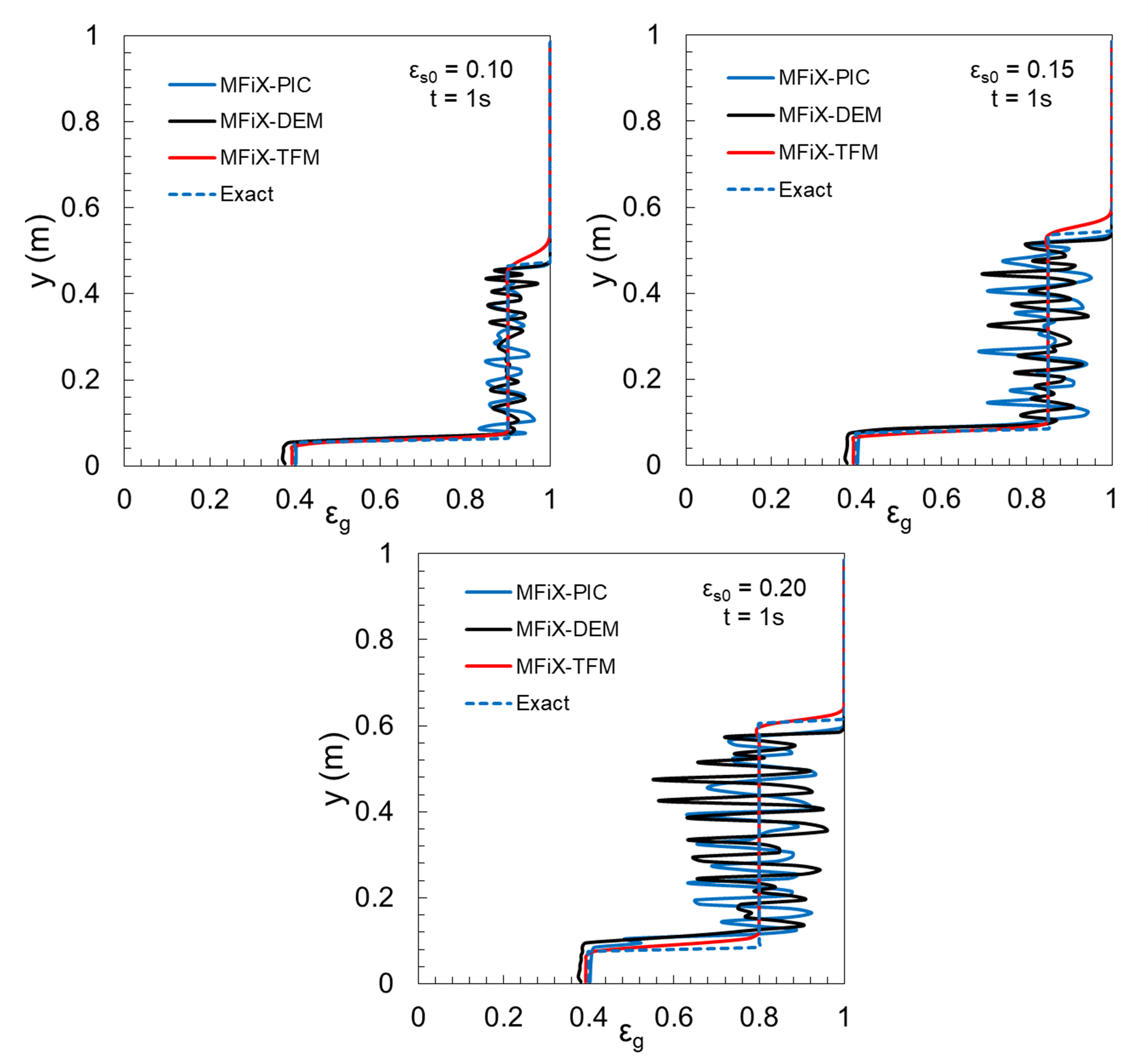
Fig. 5.4 Solutions for different initial particle concentrations: (a) 0.10, (b) 0.15, (c) 0.20.

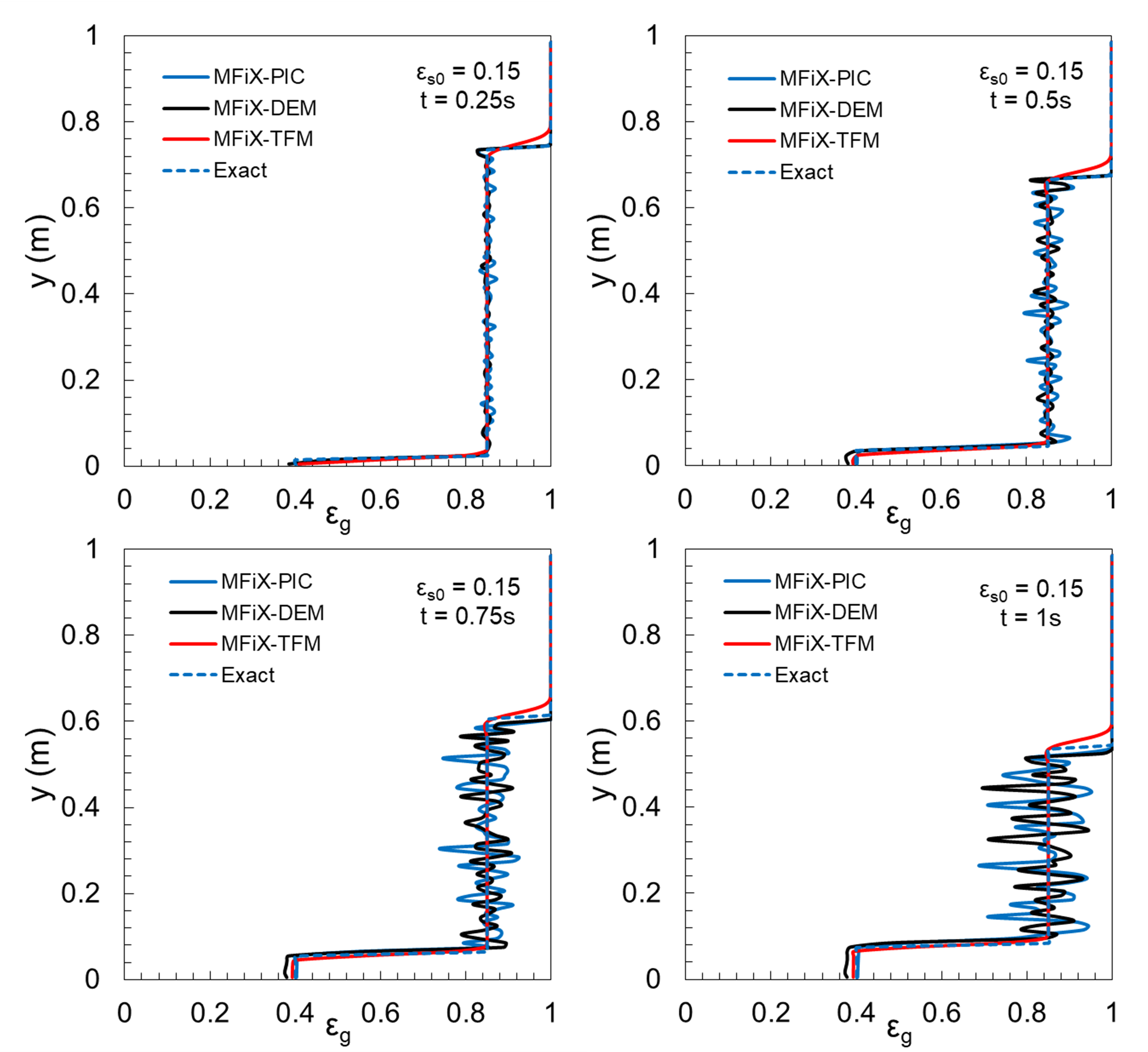
Fig. 5.5 Time evolution of shock fronts with 0.15 initial concentration.