5.6. PIC06: Rayleigh-Taylor Instability
5.6.1. Description
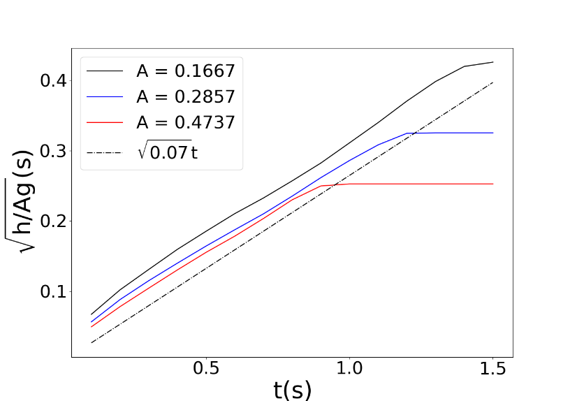
The simulation of Rayleigh-Taylor instability using PIC methodology follows the work of Snider [29]. The domain is initialized with a lighter phase at the bottom and a heavier phase at the top. When the simulation begins, the phases invert, and the growth of a mixing layer is recorded as a function of time. Researchers in the past have proposed the following functional form for the development of the mixing layer,
where the non-dimensional parameter, \(A\), used to characterize the system is Atwood number:
and the value of \(\alpha\) is between 0.05 and 0.07 (Youngs [35]; Linden et al. [15]; Snider and Andrews [30]). A rectangular domain (0.1 m X 0.6 m X 0.1 m) is chosen for simulating this system. The values for fluid and particle properties are borrowed from the work of Snider [29]. A larger value of particle diameter is used and the interphase drag coefficient (\(\propto 1/d_{p}\)) is scaled accordingly. The list of parameters used in this exercise are summarized in Table 5.13.
Case 1 |
Case 2 |
Case 3 |
|
|---|---|---|---|
Particle diameter (m) |
2 X 10⁻⁶ |
2 X 10⁻⁶ |
2 X 10⁻⁶ |
Particle density (kg/m3) |
3 |
5 |
7 |
Fluid density (kg/m3) |
1 |
1 |
1 |
Fluid viscosity (Pa-s) |
0.001 |
0.001 |
0.001 |
Atwood number |
0.1667 |
0.2857 |
0.4737 |
Drag coefficient, \(\beta\) (kg·m-3 ·s-1) |
100 \(\rho_{s} \epsilon_{s}\) |
100 \(\rho_{s} \epsilon_{s}\) |
100 \(\rho_{s} \epsilon_{s}\) |
5.6.2. Setup
Computational/Physical model |
|||
|---|---|---|---|
3D, Transient |
|||
Multiphase |
|||
Gravity |
|||
Thermal energy equation is not solved |
|||
Turbulence equations are not solved (Laminar) |
|||
Uniform mesh |
|||
First order upwind discritization scheme |
|||
Geometry |
|||
Coordinate system |
Cartesian |
Grid partitions |
|
x-length |
0.10 |
(m) |
40 |
y-length |
0.60 |
(m) |
240 |
z-length |
0.10 |
(m) |
40 |
Material |
|||
Gas density, \(\rho_{g}\) |
1.0 |
(kg·m-3) |
|
Gas viscosity, \(\mu_{g}\) |
1.8E-5 |
(Pa·s) |
|
Solids Type |
PIC |
||
Diameter, \(d_{p}\) |
0.001 |
(mm) |
|
Density, \(\rho_{s}\) |
(kg·m-3) |
||
Solids Properties (PIC) |
|||
Pressure linear scale factor, \(P_{s}\) |
1.0 |
(Pa) |
|
Exponential scale factor, \(\gamma\) |
4.0 |
(-) |
|
Statistical weight |
7.2E+08 |
(-) |
|
Initial Conditions |
|||
x-velocity, \(u_{g}\) |
0.0 |
(m·s-1) |
|
y-velocity, \(v_{g}\) |
0.0 |
(m·s-1) |
|
z-velocity, \(w_{g}\) |
0.0 |
(m·s-1) |
|
Gas volume fraction, \(\epsilon_{g}\) |
0.80 |
(-) |
|
Gas volume fraction at packing, \(\epsilon_{g}^{*}\) |
0.4 |
(-) |
|
Pressure, \(P_{g}\) |
101,325 |
(Pa) |
|
Boundary Conditions |
|||
Top boundary |
Pressue outflow |
||
All other boundaries |
Free-slip walls |
5.6.3. Results
The contour plots Fig. 5.7 show the evolution of volume fraction fields at the end of 1 second. The instability is triggered by a non-homogenous solids concentration field due to inherent randomness in generating the parcels. The instability is more pronounced at higher values of A. Fig. 5.8 shows the time evolution of the mixing layer, where the coordinates used by Snider [29] are used. The results are consistent with the work of Snider [29]. The analytical value for the slope of this curve based on Eq.5.10 is \(\sqrt{\alpha}\), which is matched reasonably well by MFiX-PIC. As A increases, the particles reach the bottom of the domain sooner resulting in the associate curve reaching a plateau.
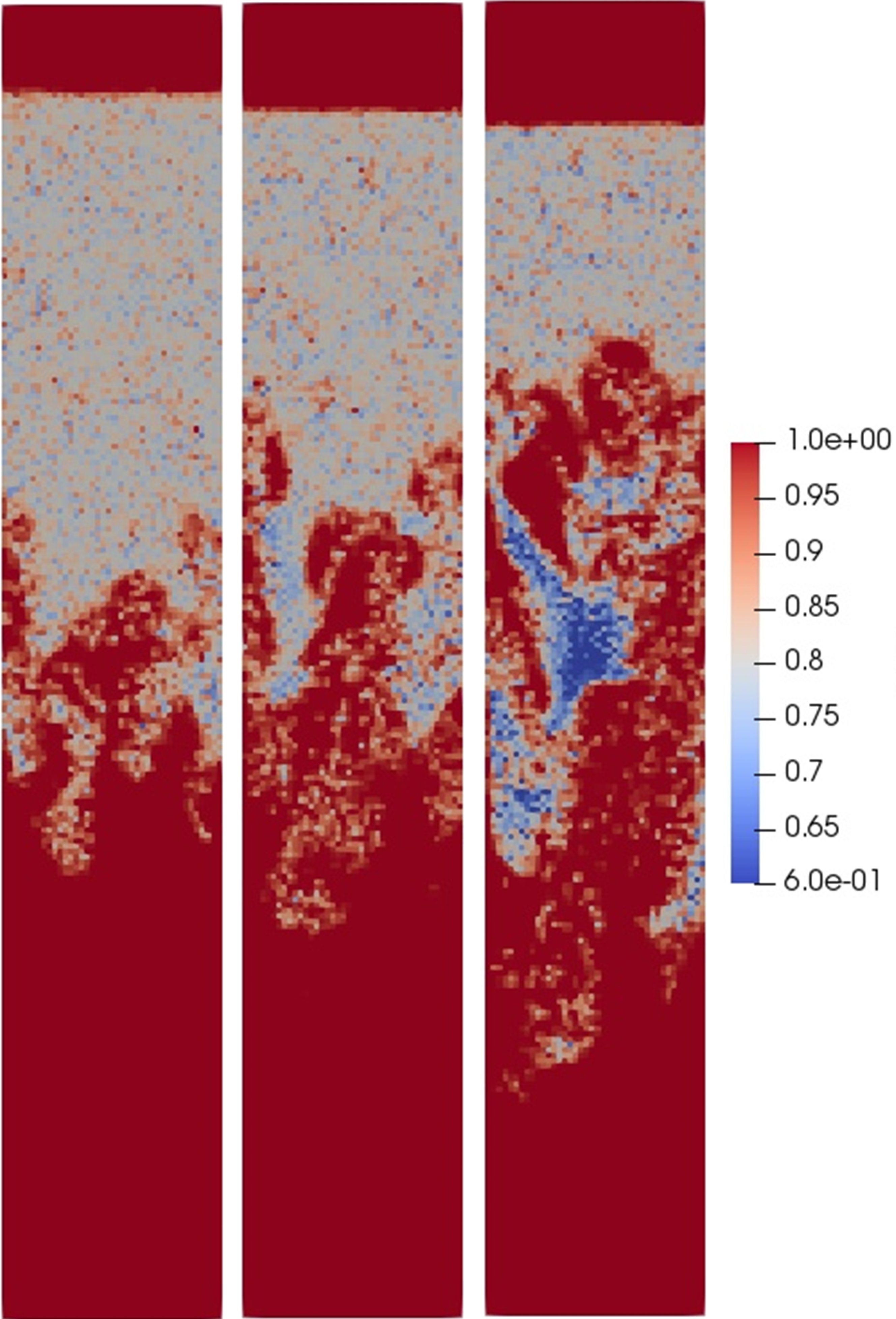
Fig. 5.7 Sectional view of volume fraction contour of the lighter phase at t = 0.8s; A = 0.1667, 0.2857, and 0.4737 (left to right)