3.1. FLD01: Steady, 2D Poiseuille flow¶

3.1.1. Description¶

Plane Poiseuille flow is defined as a steady, laminar flow of a viscous fluid between two horizontal parallel plates separated by a distance, $H$ . Flow is induced by a pressure gradient across the length of the plates, $L$ , and is characterized by a 2D parabolic velocity profile symmetric about the horizontal mid-plane as illustrated in Fig. 3.1.

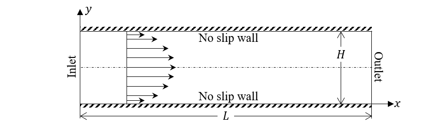
Fig. 3.1 Plane Poiseuille flow between two flat plates of length L, separated by a distance H.¶

In this problem, the Navier-Stokes equations reduce to a second order, linear, ordinary differential equation (ODE),

(3.1)¶

$\mu_{g}\frac{d^{2}u_{g}}{dy^{2}} = \frac{dP_{g}}{\text{dx}},$

where $\mu_{g}$ and $P_{g}$ are correspondingly the fluid viscosity and pressure, and $u_{g}$ and $v_{g}$ are respectively the $x$ and $y$ velocity components. Furthermore, it is assumed that gravitational forces are negligible, the pressure gradient is constant, i.e., $dP_{g}/dx = C$ , and all velocity components are zero at the channel walls. The resulting analytical solution to Eq.3.1 is given as

(3.2)¶

$u_{g}\left( y \right) = - \frac{dP_{g}}{\text{dx}}\frac{1}{2\mu_{g}}y\left( H - y \right).$

3.1.2. Setup¶

########################################################################
#                                                                      #
# Author: Aniruddha Choudhary                           Date: Jan 2015 #
# Horizontal channel (rectangular plane Poiseuille flow)               #
#                                                                      #
# A pressure gradient is imposed over x-axis cyclic boundaries. The    #
# north and south walls are no-slip.                                   #
#                                                                      #
########################################################################

  RUN_NAME = 'FLD01'
  DESCRIPTION = 'Steady, 2D Poiseuille Flow'

#_______________________________________________________________________
# RUN CONTROL SECTION

  UNITS = 'SI'
  RUN_TYPE = 'NEW'


  ENERGY_EQ =     .F.
  SPECIES_EQ(0) = .F.

  GRAVITY = 0.0

  CALL_USR = .T.

#_______________________________________________________________________
# NUMERICAL SECTION

  MAX_NIT =    200000
  TOL_RESID =   1.0E-10

  LEQ_PC(1:9) = 9*'NONE'

  DISCRETIZE(1:9) = 9*2
  NORM_G = 0.0

#_______________________________________________________________________
# GEOMETRY SECTION

  COORDINATES = 'CARTESIAN'

  ZLENGTH = 1.00     NO_K = .T.
  XLENGTH = 0.20     IMAX = 8
  YLENGTH = 0.01     JMAX = 8

#_______________________________________________________________________
# GAS-PHASE SECTION

  RO_g0 = 1.0     ! (kg/m3)
  MU_g0 = 1.0d-3  ! (Pa.s)

#_______________________________________________________________________
# SOLIDS-PHASE SECTION

  MMAX = 0

#_______________________________________________________________________
# INITIAL CONDITIONS SECTION

  IC_X_w(1) =    0.00    ! (m)
  IC_X_e(1) =    0.20    ! (m)
  IC_Y_s(1) =    0.00    ! (m)
  IC_Y_n(1) =    0.01    ! (m)

  IC_EP_g(1) =   1.0

  IC_P_g(1) =    0.0     ! (Pa)

  IC_U_g(1) =   10.0     ! (m/sec)
  IC_V_g(1) =    0.0     ! (m/sec)

#_______________________________________________________________________
# BOUNDARY CONDITIONS SECTION

! Inlet and outlet: Periodic BC
!---------------------------------------------------------------------//

  CYCLIC_X_PD = .T.
  DELP_X =     240.00    ! (Pa)

! Top and bottom walls: No-slip
!---------------------------------------------------------------------//
! Bottom wall
  BC_X_w(3) =    0.00    ! (m)
  BC_X_e(3) =    0.20    ! (m)
  BC_Y_s(3) =    0.00    ! (m)
  BC_Y_n(3) =    0.00    ! (m)

  BC_TYPE(3) = 'NSW'

! Top wall
  BC_X_w(4) =    0.00    ! (m)
  BC_X_e(4) =    0.20    ! (m)
  BC_Y_s(4) =    0.01    ! (m)
  BC_Y_n(4) =    0.01    ! (m)

  BC_TYPE(4)  = 'NSW'

#_______________________________________________________________________
# OUTPUT CONTROL SECTION

  RES_DT =        1.0    ! (sec)
  SPX_DT(1:9) = 9*1.0    ! (sec)

  FULL_LOG = .T.

  RESID_STRING  = 'P0', 'U0', 'V0'

#_______________________________________________________________________
# DMP SETUP

!  NODESI =  1  NODESJ =  1  NODESK =  1

3.1.3. Results¶

The analytical and numerical solutions for x-velocity, $u_{g}$ , are shown in Fig. 3.2. Only a subset of the numerical solution data points are plotted causing the appearance of a slight shift in presented data points. The observed error demonstrates a second-order rate of convergence with respect to grid size in the y-axial direction. This is attributed to the second-order discretization of the viscous stress term as convection/diffusion terms do not contribute to the solution.

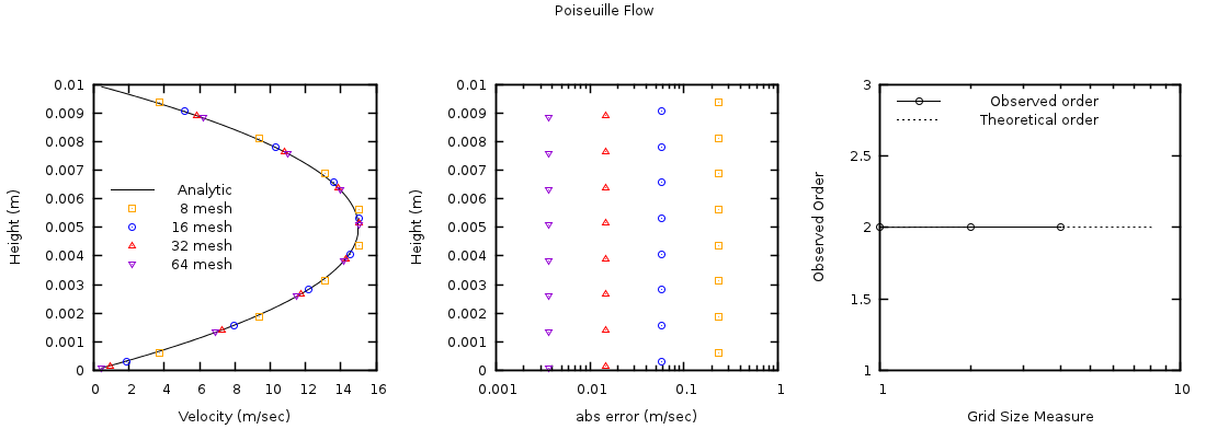
Fig. 3.2 Steady, 2D channel flow x-velocity profile (left), absolute error in x-velocity solution (center), and observed order of accuracy (right) using four grid levels (JMAX = 8, 16, 32, 64).¶

The fluid pressure, $P_{g}$ , varies linearly along the length of the plates as shown in Fig. 3.3. The largest observed absolute error is bounded above by $10^{- 12}$ and occurs for the finest mesh. This error is attributed to the convergence criteria of the linear equation system.

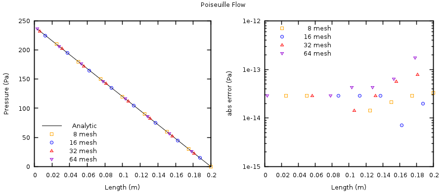
Fig. 3.3 Steady, 2D channel flow pressure profile (left) and absolute error in pressure solution (right) using four grid levels (IMAX = 8, 16, 32, 64).¶