3.3. FLD03: Steady, lid-driven square cavity
3.3.1. Description
Lid-driven flow in a 2D square cavity in the absence of gravity is illustrated in Fig. 3.6. The problem definition follows the work of Ghia et al. [10] where the domain is bounded on three sides with stationary walls while one wall, the lid, is prescribed a constant velocity. The cavity is completely filled with a fluid of selected viscosity and the flow is assumed to be incompressible and laminar.

Fig. 3.6 Schematic of the lid-driven square cavity.
3.3.2. Setup
########################################################################
#                                                                      #
# Author: M. Syamlal                                    Date: Dec 1999 #
# Revised: A. Choudhary and J. Musser                   Date: Jun 2015 #
#                                                                      #
# A top wall driven cavity with only fluid phase present in the        #
# absence of gravitational forces.                                     #
#                                                                      #
# REF: Ghia U., Ghia K.N., and Shin C.T., High-Re Solutions for Incom- #
#      pressible Flow Using the Navier-Stokes Equations and a Multi-   #
#      grid Method, Journal of Computational Physics, Volume 48, pages #
#      387-411, 1982. doi: 10.1016/0021-9991(82)90058-4                #
#                                                                      #
########################################################################

  RUN_NAME = 'FLD03'
  DESCRIPTION = 'Lid-driven cavity'

#_______________________________________________________________________
# RUN CONTROL SECTION

  UNITS = 'SI'
  RUN_TYPE = 'NEW'

  TSTOP = 1.0d8

  DT =     1.0e-2
  DT_FAC = 1.0

  ENERGY_EQ =     .F.
  SPECIES_EQ(0) = .F.

  GRAVITY = 0.0

  CALL_USR = .T.

#_______________________________________________________________________
# NUMERICAL SECTION

  LEQ_PC(1:9) = 9*'DIAG'

  DISCRETIZE(1:9) = 9*2
  DETECT_STALL = .F.

  NORM_G = 1.0

#_______________________________________________________________________
# GEOMETRY SECTION

  COORDINATES   = 'CARTESIAN'

  ZLENGTH = 1.0   NO_K = .T.
  XLENGTH = 1.0   IMAX = 128
  YLENGTH = 1.0   JMAX = 128

#_______________________________________________________________________
# GAS-PHASE SECTION

  RO_G0 = 1.0     ! (kg/m3)
  MU_G0 = 0.01    ! (Pa.sec)

#_______________________________________________________________________
# SOLIDS-PHASE SECTION

  MMAX = 0

#_______________________________________________________________________
# INITIAL CONDITIONS SECTION

  IC_X_w(1) =    0.00  ! (m)
  IC_X_e(1) =    1.00  ! (m)
  IC_Y_s(1) =    0.00  ! (m)
  IC_Y_n(1) =    1.00  ! (m)

  IC_EP_g(1) =   1.00

  IC_U_g(1) =   -1.0e-2! (m/sec)
  IC_V_g(1) =    0.00  ! (m/sec)

#_______________________________________________________________________
# BOUNDARY CONDITIONS SECTION

! West, East and South are default No-Slip Walls (NSW)

! North: Lid with a constant velocity of 1.0 m/s along +x using a
! partial slip wall (PSW) implemented as dv/dn + Hw(V-Vw) = 0.0
! where Vw is the wall speed and Hw is undefined (Inf).
!---------------------------------------------------------------------//
  BC_X_w(1) =   0.00  ! (m)
  BC_X_e(1) =   1.00  ! (m)
  BC_Y_s(1) =   1.00  ! (m)
  BC_Y_n(1) =   1.00  ! (m)

  BC_TYPE(1) = 'PSW'

  BC_Uw_g(1) =  1.00  ! (m/sec)
  BC_Vw_g(1) =  0.00  ! (m/sec)


#_______________________________________________________________________
# OUTPUT CONTROL SECTION

  RES_DT =        5.0d3 ! (sec)
  SPX_DT(1:9) = 9*5.0d3 ! (sec)

  FULL_LOG = .F.

  RESID_STRING  = 'P0' 'U0' 'V0'

#_______________________________________________________________________
# DMP SETUP

!  NODESI =  1  NODESJ =  1  NODESK =  1
3.3.3. Results
Numerical solutions were obtained on a 128x128 grid mesh for Reynolds numbers of 100 and 400 by specifying fluid viscosities of 1/100 and 1/400 Pa·s, respectively. A time step of 0.01 second was used and the simulations considered converged when the average L2 Norms for the x-axis and y-axis velocity components, \(u_{g}\) and \(v_{g}\), were less than 10-8.
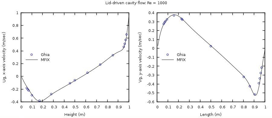
The horizontal velocity at the vertical centerline (\(x = 0.5\)) and the vertical velocity at the horizontal centerline (\(y = 0.5\)) are compared with those of Ghia et al. [10] in Fig. 3.7 and Fig. 3.8.
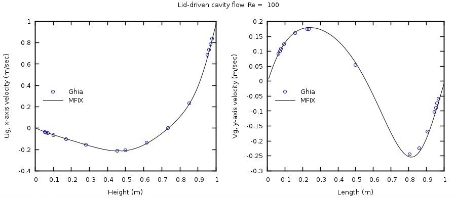
Fig. 3.7 Comparison of velocities at the vertical (x=0.5) and horizontal centerlines (y=0.5) of the cavity with Ghia et al. [10] for Reynolds number of 100 (128x128 grid).
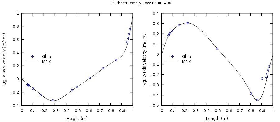
Fig. 3.8 Comparison of velocities at the vertical (x=0.5) and horizontal centerlines (y=0.5) of the cavity with Ghia et al. [10] for Reynolds number of 400 (128x128 grid).
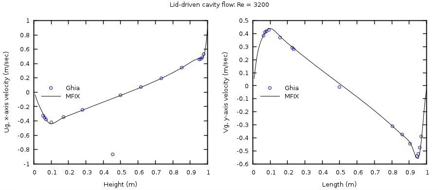
Similarly, numerical solutions were obtained on a 128x128 grid mesh for Reynolds numbers of 1000 and 3200 by specifying fluid viscosities of 1/1000 and 1/3200 Pa·s, respectively. The horizontal velocity at the vertical centerline (\(x = 0.5\)) and the vertical velocity at the horizontal centerline (\(y = 0.5\)) are compared with those of Ghia et al. [10] in Fig. 3.9 and Fig. 3.10. These cases are not included in the continuous integration server test suite.