3.4. FLD04: Gresho vortex problem
3.4.1. Description
The Gresho vortex problem [11] involves a stationary rotating vortex for which the centrifugal forces are exactly balanced by pressure gradients. The angular velocity and pressure distribution varies with radius as given by Eq.3.5,:eq:fld04eq2 [16] while the radial velocity is zero everywhere and the density is one everywhere.
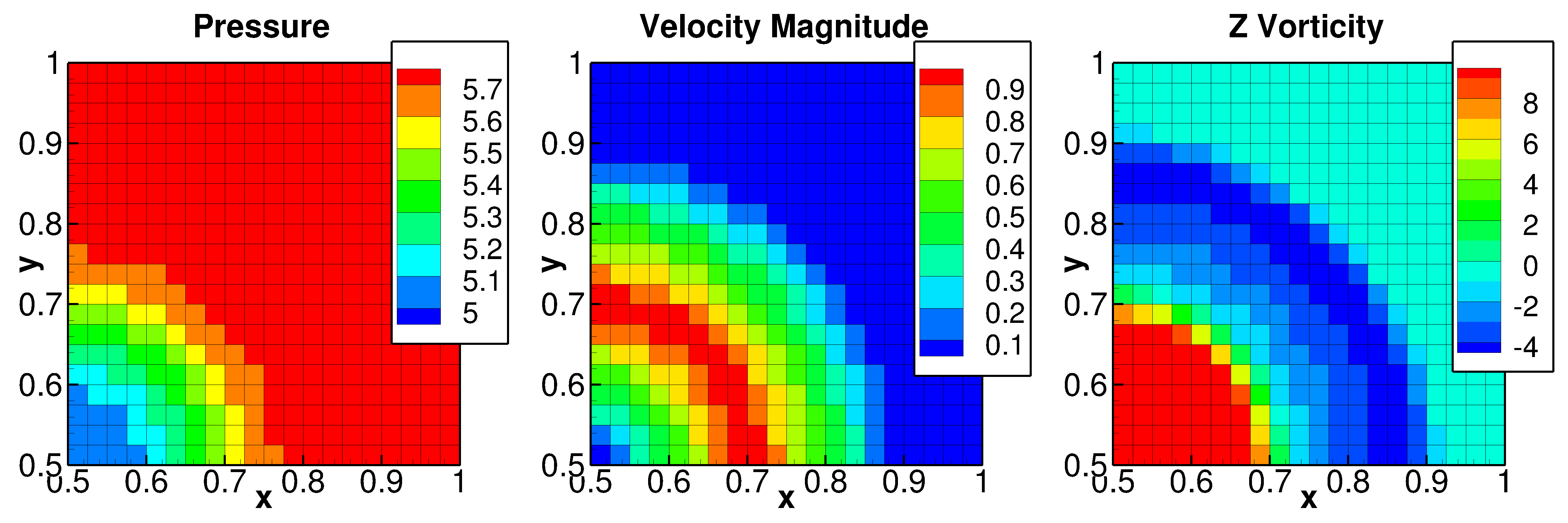
Fig. 3.11 Exact solution for the Gresho vortex problem (shown for \(\left( \mathbf{x,y} \right)\mathbf{\in}\left( \mathbf{0.5,1} \right)\mathbf{\times}\left( \mathbf{0.5,1} \right)\))
This problem is setup as a time-independent solution to the incompressible, homogeneous Euler equations. The exact solution is symmetric about the horizontal and the vertical axes and is shown for the quadrant of \(\left( x,y \right) \in \left( 0.5,1 \right) \times \left( 0.5,1 \right)\) in Figure 3‑11, where \(\left( 0.5,0.5 \right)\) is the center of the vortex. The simulation is initialized with the exact solution and periodic conditions on all boundaries of a 2D domain of unit dimensions (i.e., \(\left( x,y \right) \in \left( 0,1 \right) \times \left( 0,1 \right)\))). Different numerical schemes in MFIX are used to find the numerical solution after three seconds which are then compared with an exact solution to assess the quality of the results.
3.4.2. Setup
########################################################################
#                                                                      #
# Author: Aniruddha Choudhary                           Date: Jun 2015 #
# Gresho problem: A stationary rotating vortex.                        #
#                                                                      #
# References:                                                          #
#   [1] Liska, R. & Wendroff, B. (2003). Comparison of Several         #
#   Difference Schemes on 1D and 2D Test Problems for the              #
#   Euler Equations.                                                   #
#   SIAM J. Sci. Comput., 25, 995--1017.                               #
#   doi: 10.1137/s1064827502402120                                     #
#                                                                      #
#   [2] Gresho, P. M. & Chan, S. T. (1990). On the theory of           #
#   semi-implicit projection methods for viscous incompressible flow   #
#   and its implementation via a finite element method that also       #
#   introduces a nearly consistent mass matrix.                        #
#   Part 2: Implementation.                                            #
#   International Journal for Numerical Methods in Fluids,             #
#   11, 621--659.                                                      #
#   doi: 10.1002/fld.1650110510                                        #
#                                                                      #
########################################################################

  RUN_NAME = 'FLD04'
  DESCRIPTION = 'Gresho vortex problem'

#_______________________________________________________________________
# RUN CONTROL SECTION

  UNITS = 'SI'
  RUN_TYPE = 'NEW'

  TSTOP = 3.0

  DT =     1.0e-2
  DT_FAC = 1.0

  ENERGY_EQ =     .F.
  SPECIES_EQ(0) = .F.

  GRAVITY = 0.0

  CALL_USR = .T.

#_______________________________________________________________________
# NUMERICAL SECTION

  MAX_NIT = 100000

  TOL_RESID =  1.0e-4

  LEQ_PC(1:9) = 9*'DIAG'


#_______________________________________________________________________
# GEOMETRY SECTION

  COORDINATES  = 'CARTESIAN'

  ZLENGTH = 1.0    NO_K = .T.
  XLENGTH = 1.0    IMAX = 40
  YLENGTH = 1.0    JMAX = 40

#_______________________________________________________________________
# GAS-PHASE SECTION

  RO_G0 = 1.0     ! (kg/m3)
  MU_G0 = 0.0     ! (Pa.sec)

#_______________________________________________________________________
# SOLIDS-PHASE SECTION

  MMAX = 0

#_______________________________________________________________________
# INITIAL CONDITIONS SECTION

  IC_X_w(1) =    0.00  ! (m)
  IC_X_e(1) =    1.00  ! (m)
  IC_Y_s(1) =    0.00  ! (m)
  IC_Y_n(1) =    1.00  ! (m)

  IC_EP_g(1) =   1.00

  IC_U_g(1) =    1.00  ! (m/sec)
  IC_V_g(1) =    0.00  ! (m/sec)

#_______________________________________________________________________
# BOUNDARY CONDITIONS SECTION

! West, East, South, and North: Periodic BCs
!---------------------------------------------------------------------//

  CYCLIC_X    = .T.
  CYCLIC_Y    = .T.


#_______________________________________________________________________
# OUTPUT CONTROL SECTION

  RES_DT =        0.1   ! (sec)
  SPX_DT(1:9) = 9*0.1   ! (sec)

  FULL_LOG = .T.

  RESID_STRING  = 'P0' 'U0' 'V0'

#_______________________________________________________________________
# DMP SETUP

!  NODESI =  1  NODESJ =  1  NODESK =  1
3.4.3. Results
MFIX simulations of the Gresho vortex problem were carried out with nine spatial discretization schemes. The final flow vorticity is illustrated in Fig. 3.12 with the exact vorticity provided for reference at left. FOUP and FOUP using downwind factors are identical as expected, therefore only results for FOUP are shown. FOUP clearly fails to capture the vorticity distribution over the entire domain; Minmod and QUICKEST fail to accurately capture this distribution in the region of \(0.1\ m \leq r \leq 0.3\ m\) (e.g., \(0.6m \leq x \leq 0.8m\) along \(y = 0.5\)).
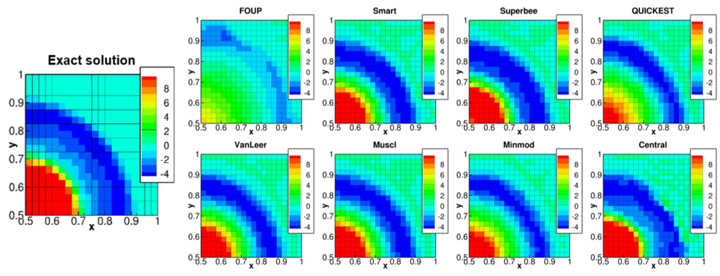
Fig. 3.12 Comparison of vorticity by different numerical schemes with the exact solution (at \(\mathbf{T = 3\ s}\)).
The total kinetic energy of the flow is included in Table 3.2. FOUP has the greatest loss of kinetic energy, followed by QUICKEST, and Minmod. Central scheme maintains the best agreement followed by SMART and MUSCL.
Scheme |
Calculated TKE |
Abs. Error |
% Rel. Error |
|---|---|---|---|
FOUP |
42.64 |
91.25 |
68.15 |
FOUP w/DWF |
42.64 |
91.25 |
68.15 |
Superbee |
144.57 |
10.66 |
7.69 |
SMART |
130.46 |
3.44 |
2.57 |
QUICKEST |
93.47 |
40.43 |
30.19 |
MUSCL |
128.45 |
5.45 |
4.07 |
van Leer |
125.79 |
8.11 |
6.05 |
Minmod |
112.95 |
20.94 |
15.64 |
Central |
133.70 |
0.20 |
0.15 |
As a final measure of solution accuracy, the average L2 Norm is shown in Table 3‑3. Again, FOUP, QUICKEST, and Minmod demonstrate greatest amount of solution error whereas Central, SMART, and Superbee have the least amount of error.
Scheme |
\(P_{g}\) L 2-norm |
\(U_{g}\) L 2-norm |
\(V_{g}\) L 2-norm |
|---|---|---|---|
FOUP |
0.1430 |
0.1468 |
0.1468 |
FOUP w/DWF |
0.1430 |
0.0822 |
0.0822 |
Superbee |
0.0184 |
0.0182 |
0.0182 |
SMART |
0.0078 |
0.0163 |
0.0163 |
QUICKEST |
0.0647 |
0.0612 |
0.0612 |
MUSCL |
0.0109 |
0.0200 |
0.0200 |
van Leer |
0.0149 |
0.0107 |
0.0107 |
Minmod |
0.0343 |
0.0408 |
0.0408 |
Central |
0.0076 |
0.0161 |
0.0161 |