3.5. FLD05: Steady, 2D Couette flow
3.5.1. Description
Couette flow is a laminar flow of a viscous fluid between two parallel plates separated by a distance, \(H\), with the upper wall moving at velocity, \(U\). Different velocity distributions are obtained depending on the pressure gradient applied to the flow field. The schematic of the problem is shown in Fig. 3.13.
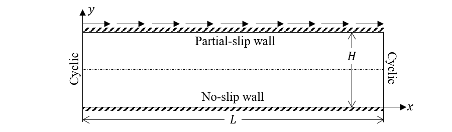
Fig. 3.13 Couette flow between two flat plates of length L, separated by a distance H with the upper wall moving at velocity U.
In this problem, the Navier-Stokes equations reduce to a second order, linear, ordinary differential equation (ODE),
where \(\mu_{g}\) is the fluid viscosity, and \(\text{dp}/\text{dx}\) is the prescribed pressure drop across the length of the pipe. The no-slip and partial-slip boundary conditions are specified by
The analytical solution is given by,
3.5.2. Setup
#########################################################################
#                                                                       #
# Author: Avinash Vaidheeswaran                         Date: July 2016 #
# Couette flow problem:                                                 #
#                                                                       #
# The south wall is held stationary and the north wall moves with a     #
# velocity U. Cyclic boundary conditions along x direction with         #
# adverase, zero, and favorable pressure gradients.                     #
#                                                                       #
#########################################################################

  RUN_NAME      = 'FLD05'
  DESCRIPTION   = 'Couette flow test cases'

#_______________________________________________________________________
# RUN CONTROL SECTION

  UNITS = 'SI'
  RUN_TYPE = 'NEW'

  ENERGY_EQ =     .F.
  SPECIES_EQ(0) = .F.

  GRAVITY = 0.0

  CALL_USR = .T.

#_______________________________________________________________________
# NUMERICAL SECTION

  MAX_NIT = 50000
  TOL_RESID = 1.0E-10

  LEQ_PC = 9*'NONE'

#_______________________________________________________________________
# GEOMETRY SECTION

  COORDINATES   = 'CARTESIAN'

  XLENGTH = 1.00     IMAX =  3
  ZLENGTH = 1.00     NO_K = .T.

  YLENGTH = 0.01     JMAX = 8

#_______________________________________________________________________
# GAS-PHASE SECTION

  RO_g0 = 1.00      ! (kg/m3)
  MU_g0 = 5.00d-6   ! (Pa.s)

#_______________________________________________________________________
# SOLIDS-PHASE SECTION

  MMAX = 0

#_______________________________________________________________________
# INITIAL CONDITIONS SECTION

  IC_X_w(1) =   0.00  ! (m)
  IC_X_e(1) =   1.00  ! (m)
  IC_Y_s(1) =   0.00  ! (m)
  IC_Y_n(1) =   0.01  ! (m)

  IC_EP_g(1) =  1.00

  IC_P_g(1) =   0.00  ! (Pa)

  IC_U_g(1) =   0.00  ! (m/sec)
  IC_V_g(1) =   0.00  ! (m/sec)

#_______________________________________________________________________
# BOUNDARY CONDITIONS SECTION


! The north was has a constant velocity of 10.0 m/s, and is set using
! a partial slip wall (PSW):  dU/dn + hw(U-Uw) = 0 where Uw = 10.0 m/s
! and hw=unsepcified (i.e., no-slip moving wall).
!---------------------------------------------------------------------//
  BC_X_w(1) =   0.00  ! (m)
  BC_X_e(1) =   1.00  ! (m)
  BC_Y_s(1) =   0.01  ! (m)
  BC_Y_n(1) =   0.01  ! (m)

  BC_TYPE(1)  = 'PSW'

  BC_Uw_g(1) = 10.00   ! (m/sec)
  BC_Vw_g(1) =  0.00   ! (m/sec)


! The south wal is a stational no-slip wall (NSW).
!---------------------------------------------------------------------//
  BC_X_w(2) =   0.00  ! (m)
  BC_X_e(2) =   1.00  ! (m)
  BC_Y_s(2) =   0.00  ! (m)
  BC_Y_n(2) =   0.00  ! (m)

  BC_TYPE(2) =  'NSW'


! The east and west boundareis are set a runtime as cyclic with a
! specified pressure drop (DELP_X)
!---------------------------------------------------------------------//
  CYCLIC_X_PD = .TRUE.
  DELP_X =  -3.0


#_______________________________________________________________________
# OUTPUT CONTROL SECTION

  RES_DT      = 1.
  FULL_LOG    = .T.
  SPX_DT      = 9*1.

  RESID_STRING  = 'P0' 'U0' 'V0'

#_______________________________________________________________________
# DMP SETUP
3.5.3. Results
Simulations were conducted for seven pressure drops, \(\lbrack - 3.0,\ - 2.0,\ - 1.0,\ \ 0.0,\ 1.0,\ 2.0,\ 3.0\rbrack\) Pa, specified across the x-axial cyclic boundaries. Four mesh levels [8, 16, 32, 64] in the y-axial direction were used to assess discretization error.
The analytical and numerical solutions for the zero pressure drop case are shown in Fig. 3.14. For clarity, only a subset of the numerical solutions is presented, resulting in a slight offset/shift in displayed data points. Note that the analytical solution reduces to a linear variation in velocity between the lower and upper walls when the specified pressure drop is zero. For this case, the absolute error in velocity is bounded above by \(10^{- 6}\ \mathrm{m \cdot sec}^{- 1}\) and is observed for the finest grid resolution (64 mesh). Further investigation (not presented) indicated that the increase in numerical error is attributed to the solution mechanism of the linear equation system. This error can be reduced by modifying the default linear equation solver settings (e.g., tighten convergence criteria, increase number of iterations, etc.).
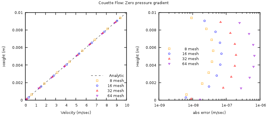
Fig. 3.14 Couette flow with a zero pressure gradient with four grid resolutions.
The analytical and numerical solutions for the adverse and favorable pressure drops are shown in Fig. 3.15 and Fig. 3.16. Again, only a subset of the numerical solutions is presented resulting in a slight offset/shift in displayed data points. These cases demonstrate a second order rate of convergence with respect to grid size which is attributed to the second-order discretization of the viscous stress term.
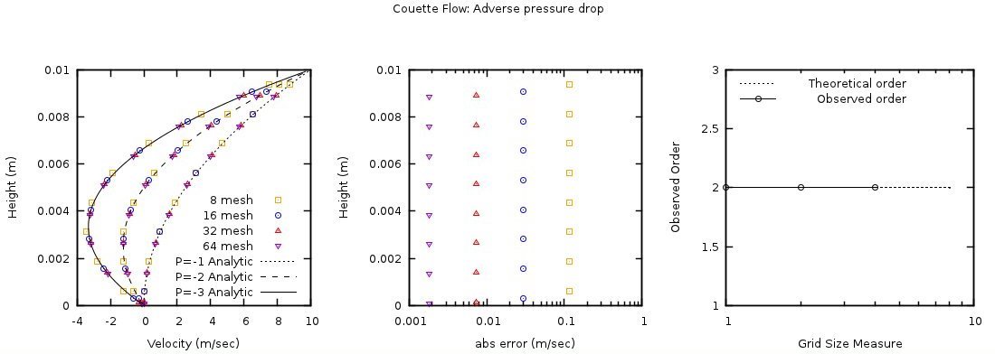
Fig. 3.15 Adverse pressure gradient (-1, -2, -3 Pa) Couette flow with four grid resolutions. Absolute error and observed order of accuracy only shown for -3 Pa pressure gradient.
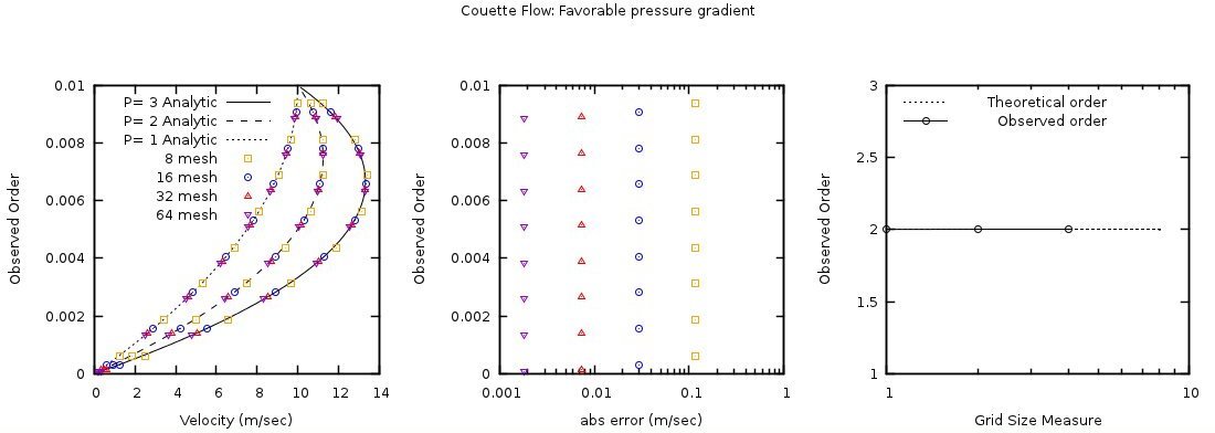
Fig. 3.16 Favorable pressure gradient (1, 2, 3 Pa) Couette flow with four grid resolutions. Absolute error and observed order of accuracy only shown for 3 Pa pressure gradient.