3.8. FLD08: Steady, 2D turbulent pipe flow
3.8.1. Description
This case uses turbulent flow in a pipe of length \(L\) and radius \(R\) to assess the single phase k-ϵ model in MFIX. A 2D axisymmetric domain is used to define the pipe geometry, and pressure boundaries are used to induce flow in the positive y-axial direction as shown in Fig. 3.20. The results are compared with the experimental data of Zagarola and Smits [36].
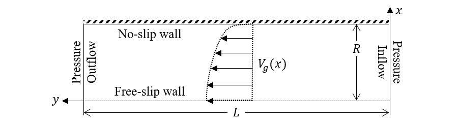
Fig. 3.20 Turbulent flow in a pipe
3.8.2. Setup
#########################################################################
#                                                                       #
# Author: Avinash Vaidheeswaran                         Date: July 2016 #
# Turbulent flow in a pipe problem:                                     #
#                                                                       #
# Turbulent flow through a pipe is simulated and the results are        #
# compared with the data from Princeton superpipe.                      #
#                                                                       #
# Data source, accessed November, 2016                                  #
# http://www.princeton.edu/~gasdyn/Superpipe_data/4.1727E+04.txt        #
#                                                                       #
#       -*-*-*-*-*-*-*-*-*-*-* FSW 3 *-*-*-*-*-*-*-*-*-*-*-*-           #
#      -1->                                               -2->          #
#   PI -1->                                               -2-> PO       #
#      -1->                                               -2->          #
#       ---------------------- NSW 4 ------------------------           #
#                                                                       #
#########################################################################

  RUN_NAME = 'FLD08'
  DESCRIPTION = 'Pipe flow case'

#_______________________________________________________________________
# RUN CONTROL SECTION

  UNITS = 'SI'
  RUN_TYPE = 'NEW'

  TSTOP = 1.0d8

  DT =     0.1
  DT_FAC = 1.0

  ENERGY_EQ  = .F.
  SPECIES_EQ = .F.

  GRAVITY = 0.0

  CALL_USR = .T.

#_______________________________________________________________________
# NUMERICAL SECTION

  DETECT_STALL = .F.

  NORM_g = 0.0

#_______________________________________________________________________
# GEOMETRY SECTION

  COORDINATES   =   'CYLINDRICAL'

  ZLENGTH = 6.23819  NO_K =  .T.
  XLENGTH = 0.06468  IMAX =  16
  YLENGTH = 8.00     JMAX = 100

#_______________________________________________________________________
# GAS-PHASE SECTION

  RO_g0 = 1.1620      ! (kg/m3)
  MU_g0 = 1.8487d-05  ! (Pa.s)

  TURBULENCE_MODEL = 'K_EPSILON'

  MU_GMAX = 1.0d6     ! (Pa.s)

#_______________________________________________________________________
# SOLIDS-PHASE SECTION

  MMAX = 0

#_______________________________________________________________________
# INITIAL CONDITIONS SECTION

  IC_X_w(1) =      0.00     ! (m)
  IC_X_e(1) =      0.06468  ! (m)
  IC_Y_s(1) =      0.00     ! (m)
  IC_Y_n(1) =      8.00     ! (m)

  IC_EP_G(1) =     1.00     ! (-)

  IC_P_G(1) =      0.00     ! (Pa)

  IC_U_G(1) =      0.00     ! (m/sec)
  IC_V_G(1) =      5.00     ! (m/sec)

  IC_K_TURB_G(1) = 0.047    ! (m2/s2)
  IC_E_TURB_G(1) = 0.213    ! (m2/s3)

#_______________________________________________________________________
# BOUNDARY CONDITIONS SECTION

! The south boundary is a pressure inflow
!---------------------------------------------------------------------//
  BC_X_w(1) =      0.00      ! (m)
  BC_X_e(1) =      0.06468   ! (m)
  BC_Y_s(1) =      0.00      ! (m)
  BC_Y_n(1) =      0.00      ! (m)

  BC_TYPE(1) =     'PI'

  BC_EP_g(1) =     1.0       ! (-)

  BC_P_g(1) =     20.684     ! (Pa)

  BC_K_TURB_G(1) = 0.047     ! (m2/s2)
  BC_E_TURB_G(1) = 0.213     ! (m2/s3)


! The north boundary is a pressure outlet.
!---------------------------------------------------------------------//

  BC_X_w(2) =      0.00      ! (m)
  BC_X_e(2) =      0.06468   ! (m)
  BC_Y_s(2) =      8.00      ! (m)
  BC_Y_n(2) =      8.00      ! (m)

  BC_TYPE(2) =     'PO'

  BC_P_g(2) =      0.00      ! (Pa)


! The west boundary is a free-slip walls (FSW)
!---------------------------------------------------------------------//

  BC_X_w(3) =      0.00      ! (m)
  BC_X_e(3) =      0.00      ! (m)
  BC_Y_s(3) =      0.00      ! (m)
  BC_Y_n(3) =      8.00      ! (m)

  BC_TYPE(3) =  'FSW'


! The east boundary is a no-slip wall (NSW)
!---------------------------------------------------------------------//

  BC_X_w(4) =      0.06468   ! (m)
  BC_X_e(4) =      0.06468   ! (m)
  BC_Y_s(4) =      0.00      ! (m)
  BC_Y_n(4) =      8.00      ! (m)

  BC_TYPE(4) =  'NSW'


#_______________________________________________________________________
# OUTPUT CONTROL SECTION

  RES_DT = 1.0d8
  SPX_DT(1:9) = 9*1.0d8

  FULL_LOG = .F.
  RESID_STRING = 'P0' 'U0' 'V0' 'K0'


#_______________________________________________________________________
# DMP SETUP

!  NODESI =  1  NODESJ =  1  NODESK =  1
3.8.3. Results
Pressure drop in the y-axial direction, domain width, gas density and viscosity were chosen to reflect the conditions of [36] for \(Re = 41727\). A transient simulation was performed for better numerical stability. The solution was considered converged when the L2 norms for the gas velocity components, \(u_{g}\) and \(v_{g}\), turbulent kinetic energy, \(k_{g}\), and rate of turbulent kinetic energy dissipation, \(\epsilon_{g}\), were all less than 10-10.
The simulation was conducted with 16 cells in the x-axial direction. The mesh level ensures that the stream-ways velocity components in computational cells adjacent to the wall were located outside the buffer layer. Specifically, the first stream-ways velocity component was located at least 30 wall units from the wall to be consistent with the \(k - \epsilon\) model wall function implementation.
Here, the friction velocity, \(v_{*}\), is given by the Karman number, \(R^{+}\) [36],
where \(D\) is pipe diameter, and \(\nu\) is the kinematic viscosity.
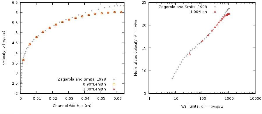
The MFIX results are shown in Fig. 3.21 along with the experimental data of Zagarola and Smits [36] for \(Re = 41727\). The experimental dataset was accessed on November 10, 2016 from http://www.princeton.edu/~gasdyn/Superpipe_data/4.1727E+04.txt
The velocity profile is shown on the left, and the normalized velocity profile with respect to wall units is shown on the right. The velocity profile is given for two locations near the pipe exit, 7.2 m and 8.0 m respectively, with the maximum difference less than 10-2 m·sec-1, indicating that the flow is fully developed. The largest discrepancy between the experimental measurements and the simulation results occurs at the centerline of the domain where the simulation under-predicts the observed velocity by 0.3 m·sec-1.