3.7. FLD07: Steady, 2D fully-developed, turbulent channel flow
3.7.1. Description
This case uses 2D, fully-developed turbulent channel flow between two horizontal, parallel plates separated by a width, \(W\), to assess the single phase k-ϵ model in MFIX. Periodic boundaries with a specified pressure drop are imposed in the y-direction as shown in Fig. 3.18.

Fig. 3.18 Turbulent flow in a 2D channel
The pressure drop along the channel is equated to the shear stress at the walls, \(\tau_{w}\).
The shear stress is related to the gas density, \(\rho_{g}\), and friction velocity, \(v_{*}\),
where, the friction velocity, is given by the Reynolds number.
3.7.2. Setup
#########################################################################
#                                                                       #
# Author: Avinash Vaidheeswaran                         Date: July 2016 #
# Turbulent flow in a pipe problem:                                     #
#                                                                       #
# Turbulent flow through a channel is simulated and the results are     #
# compared with the data from DNS                                       #
#                                                                       #
#########################################################################

  RUN_NAME = 'FLD07'
  DESCRIPTION = 'Turbulent channel flow'

#_______________________________________________________________________
# RUN CONTROL SECTION

  UNITS = 'SI'
  RUN_TYPE = 'NEW'

  TSTOP = 1.0d8

  DT = 0.02

  ENERGY_EQ =     .F.
  SPECIES_EQ(0) = .F.

  GRAVITY = 0.0

  CALL_USR = .T.

#_______________________________________________________________________
# NUMERICAL SECTION

  DISCRETIZE(1:9) = 9*2

  NORM_g = 0.0

#_______________________________________________________________________
# GEOMETRY SECTION

  COORDINATES = 'CARTESIAN'

  ZLENGTH =  1.00     NO_K = .T.
  XLENGTH =  2.00     IMAX =  8
  YLENGTH =  1.00     JMAX =  4

#_______________________________________________________________________
# GAS-PHASE SECTION

  RO_g0 = 1.0        ! (kg/m3)
  MU_g0 = 1.0d-04    ! (Pa.s)

  TURBULENCE_MODEL = 'K_EPSILON'

  MU_GMAX =  1.0d6   ! (Pa.s)

#_______________________________________________________________________
# SOLIDS-PHASE SECTION

  MMAX = 0

#_______________________________________________________________________
# INITIAL CONDITIONS SECTION

  IC_X_w(1) =      0.0     ! (m)
  IC_X_e(1) =      2.0     ! (m)
  IC_Y_s(1) =      0.0     ! (m)
  IC_Y_n(1) =      1.0     ! (m)

  IC_EP_G(1) =     1.0

  IC_P_G(1) =      0.0     ! (Pa)

  IC_U_G(1) =      1.0d-6  ! (m/sec)
  IC_V_G(1) =      1.0     ! (m/sec)

  IC_K_TURB_G(1) = 0.010   ! (m2/s2)
  IC_E_TURB_G(1) = 0.001   ! (m2/s3)

#_______________________________________________________________________
# BOUNDARY CONDITIONS SECTION

! Flow boundaries: Periodic with specified pressure drop
!---------------------------------------------------------------------//
  CYCLIC_Y_PD = .T.
  DELP_Y = @(0.0543496*0.0543496)    ! (Pa)


! The east and west boundaries are no-slip walls (NSW)
!---------------------------------------------------------------------//

  BC_X_w(1:2) =     0.0     2.0    ! (m)
  BC_X_e(1:2) =     0.0     2.0    ! (m)
  BC_Y_s(1:2) =     0.0     0.0    ! (m)
  BC_Y_n(1:2) =     1.0     1.0    ! (m)

  BC_TYPE(1:2) = 2*'NSW'


#_______________________________________________________________________
# OUTPUT CONTROL SECTION

  RES_DT = 1.0d6
  SPX_DT(1:9) = 9*1.0

  FULL_LOG = .F.
  RESID_STRING  =    'P0' 'U0' 'V0' 'K0'

#_______________________________________________________________________
# DMP SETUP

!  NODESI = 1    NODESJ = 2    NODESK = 1
3.7.3. Results
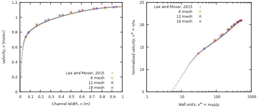
The pressure drop in the y-axial direction, domain length and width, and gas density were chosen to reflect the conditions of Lee and Moser [14] for \(\text{Re}_{\tau} = 543\). The DNS dataset was accessed on November 10, 2016 from http://turbulence.ices.utexas.edu/channel2015/data/LM_Channel_0550_mean_prof.dat.
Transient simulations were performed for better numerical stability. The solution was considered converged when the L2 norms for the gas velocity components, \(u_{g}\) and \(v_{g}\), turbulent kinetic energy, \(k_{g}\), and rate of turbulent kinetic energy dissipation, \(\epsilon_{g}\), were all less than 10-10.
Simulations were conducted for three mesh levels [6, 12, 18] in the x-axial direction. Mesh levels were selected to ensure that the stream-ways velocity components in computational cells adjacent to the wall were located outside the buffer layer. Specifically, the first stream-ways velocity component should be located at least 30 wall units from the wall to be consistent with the \(k - \epsilon\) model wall function implementation.
The MFIX results are shown in Fig. 3.19 along with the direct numerical simulation (DNS) data of Lee and Moser [14] for \(\text{Re}_{\tau} = 543\). The velocity profiles for the three mesh levels are shown on the left whereas the normalized velocity profiles with respect to wall units are shown on the right.