3.6. FLD06: Steady, 2D multi-component species transport¶

3.6.1. Description¶

The 2D multi-component species problem investigates the transport of three non-reacting fluid phase species that follow ideal gas behavior. Illustrated in Fig. 3.17, three separate mass inflows are used to inject three distinct gas species into the system. The species mix as the fluid passes through the domain such that they are well-mixed when the fluid reaches the outlet. The resulting species mass fractions, \(X_{\text{gi}}\), for the well-mixed flow are given analytically by,

(3.10)¶\[X_{\text{gi}} = \frac{\text{MW}_{\text{gi}}}{\sum_{k}^{}\text{MW}_{\text{gk}}}\]

where \(\text{MW}_{\text{gi}}\) is the molecular weight of the \(i^{\text{th}}\) gas phase species.

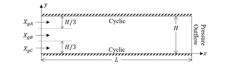
Fig. 3.17 Multicomponent species transport.¶

3.6.2. Setup¶

#########################################################################
#                                                                       #
# Author: Avinash Vaidheeswaran                         Date: July 2016 #
# Species transport problem:                                            #
#                                                                       #
# Species are introduced through mass infow BCs. The north and south    #
# boundaries are free-slip walls. The east boundary is a pressure       #
# outlet.                                                               #
#                                                                       #
#       -------------------- CYCLIC BC ----------------------           #
#   MI  -3->                                             -4->           #
#   MI  -2->                                             -4-> PO        #
#   MI  -1->                                             -4->           #
#       -------------------- CYCLIC BC ----------------------           #
#                                                                       #
#########################################################################

  RUN_NAME = 'FLD06'
  DESCRIPTION = 'Species transport test cases'

#_______________________________________________________________________
# RUN CONTROL SECTION

  UNITS =   'SI'
  RUN_TYPE = 'NEW'

  TSTOP = 10.0d6

  DT =     0.01
  DT_FAC = 1.00

  ENERGY_EQ =     .F.
  SPECIES_EQ(0) = .T.

  GRAVITY = 0.0

  CALL_USR = .T.

#_______________________________________________________________________
# NUMERICAL SECTION

  DISCRETIZE(1:9) = 9*3
  CHI_SCHEME = .T.

  NORM_G = 1.0
  DETECT_STALL = .F.

  TOL_RESID_X = 1.0d-6

#_______________________________________________________________________
# GEOMETRY SECTION

  COORDINATES   =   'CARTESIAN'

  ZLENGTH = 1.00     NO_K = .T.
  XLENGTH = 2.00     IMAX = 200
  YLENGTH = 0.03     JMAX =   3    CYCLIC_Y=.T.

#_______________________________________________________________________
# GAS-PHASE SECTION

  NMAX_g        =   3
  SPECIES_g(1)  =   'A'
  SPECIES_g(2)  =   'B'
  SPECIES_g(3)  =   'C'

  MW_g(1) =  1.0
  MW_g(2) = 10.0
  MW_g(3) = 25.0

  DIF_g0=  1.0d-3

#_______________________________________________________________________
# SOLIDS-PHASE SECTION

  MMAX = 0

#_______________________________________________________________________
# INITIAL CONDITIONS SECTION

  IC_X_w(1) =     0.00     ! (m)
  IC_X_e(1) =     2.00     ! (m)
  IC_Y_s(1) =     0.00     ! (m)
  IC_Y_n(1) =     0.03     ! (m)

  IC_EP_g(1) =    1.00     ! (1)

  IC_T_G(1) =   293.15     ! (K)
  IC_P_G(1) =   101.0d3    ! (Pa)

  IC_U_g(1) =     0.0      ! (m/sec)
  IC_V_g(1) =     0.0      ! (m/sec)

  IC_X_g(1,1) =   0.03     ! N2
  IC_X_g(1,2) =   0.27     ! H2
  IC_X_g(1,3) =   0.70     ! H2O

#_______________________________________________________________________
# BOUNDARY CONDITIONS SECTION


! The west boundary IN1 is a velocity inlet
!---------------------------------------------------------------------//
  BC_X_w(1:3) =       0.00    0.00    0.00   ! (m)
  BC_X_e(1:3) =       0.00    0.00    0.00   ! (m)
  BC_Y_s(1:3) =       0.00    0.01    0.02   ! (m)
  BC_Y_n(1:3) =       0.01    0.02    0.03   ! (m)

  BC_X_G(1:3,1) =     1.00    0.00    0.00   ! (N2)
  BC_X_G(1:3,2) =     0.00    1.00    0.00   ! (H2)
  BC_X_G(1:3,3) =     0.00    0.00    1.00   ! (H2O)

  BC_TYPE(1:3) =    3*'MI'

  BC_EP_g(1:3) =    3*1.00

  BC_T_g(1:3) =   3*293.15     ! (Pa)
  BC_P_g(1:3) =   3*101.0d3    ! (Pa)

  BC_U_g(1:3) =     3*0.25     ! (m/s)
  BC_V_g(1:3) =     3*0.00     ! (m/s)


! The east boundary is a pressure outlet.
!---------------------------------------------------------------------//

  BC_X_w(4) =    2.00    ! (m)
  BC_X_e(4) =    2.00    ! (m)
  BC_Y_s(4) =    0.00    ! (m)
  BC_Y_n(4) =    0.03    ! (m)

  BC_TYPE(4) =  'PO'

  BC_T_g(4) =  293.15    ! (K)
  BC_P_g(4) =  101.0d3   ! (Pa)


#_______________________________________________________________________
# OUTPUT CONTROL SECTION

  RES_DT =        0.1
  SPX_DT(1:9) = 9*0.1

  FULL_LOG  = .F.
  RESID_STRING  =    'P0' 'U0' 'V0'

#_______________________________________________________________________
# DMP SETUP

!  NODESI =  1  NODESJ =  1  NODESK =  1

3.6.3. Results¶

The simulation was performed using the SMART discretization scheme with the χ correction to ensure species conservation. The average L₂ norm for the three species mass fractions were calculated for consecutive time steps. The simulation was considered converged when all three norms were less than 10^-8. The species mass fractions at the outflow plane and the L₂ norm between the MFIX and analytical solution are shown in Table 3.4. Two additional simulations were carried out where the solution order of the species equations was varied (e.g., ABC, BCA, CAB). No dependence was found on the solution order of the species equations (results not shown).

Table 3.4 Average species mass fractions at the outflow and average L₂ Norms between the analytical and MFIX species mass fraction for the well-mixed fluid.¶
Species	MFiX	L ₂ norm
A	0.027778	5.86e-7
B	0.277776	2.07e-6
C	0.694446	1.48e-6