3.2. FLD02: Steady, 1D heat conduction
3.2.1. Description
Steady-state, one-dimensional heat conduction occurs across a rectangular plane-shaped slab of length \(L\) with constant material properties. As shown in Fig. 3.4, two opposing slab boundaries are maintained at constant temperatures. All other faces are perfectly insulated such that the heat flux along these boundaries is zero. Without heat generation, heat transfer through the \(x = 0\) face must equal that through the \(x = L\) face.

Fig. 3.4 Plane slab with constant material properties and no internal heat generation is shown with constant temperatures specified on opposing faces. The slab is assumed to be perfectly insulated along all other faces.
For constant thermal conductivity, the energy equation reduces to a second order ODE with Dirichlet boundary conditions as given by :eq:fld02eq1. The analytical solution for temperature distribution within the slab follows a line as given by :eq:fld02eq2.
3.2.2. Setup
########################################################################
#                                                                      #
# Author: Aniruddha Choudhary                           Date: May 2015 #
# Steady-state 1D heat conduction through a plane slab.                #
#                                                                      #
# Default walls are used for the north/south boundaries as they are    #
# adiabatic. The termperature is specified for the east/west walls.    #
########################################################################

  RUN_NAME = 'FLD02'
  DESCRIPTION = 'Steady, 1D heat conduction'

#_______________________________________________________________________
# RUN CONTROL SECTION

  UNITS = 'SI'
  RUN_TYPE = 'NEW'

  MOMENTUM_X_EQ = .F.
  MOMENTUM_Y_EQ = .F.

  ENERGY_EQ =     .T.
  SPECIES_EQ(0) = .F.

  GRAVITY = 0.0

  CALL_USR = .T.

#_______________________________________________________________________
# NUMERICAL SECTION

  Max_nit = 200000
  TOL_RESID_T = 1.0E-16

  LEQ_PC(6) = 'NONE'

#_______________________________________________________________________
# GEOMETRY SECTION

  COORDINATES   = 'CARTESIAN'

  ZLENGTH = 1.00     NO_K = .T.
  XLENGTH = 1.00     IMAX = 8
  YLENGTH = 1.00     JMAX = 8

#_______________________________________________________________________
# GAS-PHASE SECTION

  RO_g0 = 1.0   ! (kg/m3)
  MU_g0 = 1.0   ! (Pa.s)
  C_Pg0 = 1.0   ! (J/kg.K)
  K_g0 =  1.0   ! (W/m.K)

#_______________________________________________________________________
# SOLIDS-PHASE SECTION

  MMAX = 0

#_______________________________________________________________________
# INITIAL CONDITIONS SECTION

  IC_X_w(1) =    0.0     ! (m)
  IC_X_e(1) =    1.0     ! (m)
  IC_Y_s(1) =    0.0     ! (m)
  IC_Y_n(1) =    1.0     ! (m)

  IC_EP_g(1) =   1.0

  IC_P_g(1) =    0.0     ! (Pa)
  IC_T_g(1) =  350.0     ! (K)

  IC_U_g(1) =    0.0     ! (m/sec)
  IC_V_g(1) =    0.0     ! (m/sec)

#_______________________________________________________________________
# BOUNDARY CONDITIONS SECTION

! Specified temperatures at west and east walls
!---------------------------------------------------------------------//
  BC_X_w(1:2) =     0.0    1.0    ! (m)
  BC_X_e(1:2) =     0.0    1.0    ! (m)
  BC_Y_s(1:2) =     0.0    0.0    ! (m)
  BC_Y_n(1:2) =     1.0    1.0    ! (m)

  BC_TYPE(1:2) =   'NSW'  'NSW'

  BC_Tw_g(1:2) =  400.0  300.0    ! (K)


#_______________________________________________________________________
# OUTPUT CONTROL SECTION

  RES_DT =        1.0   ! (sec)
  SPX_DT(1:9) = 9*1.0   ! (sec)

  FULL_LOG    = .T.

  RESID_STRING  = 'T0'

#_______________________________________________________________________
# DMP SETUP

!  NODESI =  1  NODESJ =  1  NODESK =  1
3.2.3. Results
The analytical and numerical solutions for temperature, \(T_{g}\), are shown in Fig. 3.5. Only a subset of the numerical solution data points are plotted causing the appearance of a slight shift in presented data points. The largest observed absolute error is bounded above by \(10^{- 12}\) and occurs for the finest mesh. This error is attributed to convergence criteria of the linear equation solver.
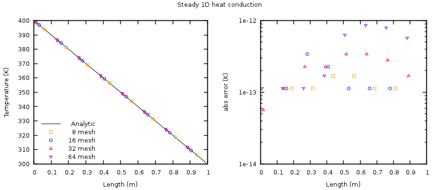
Fig. 3.5 Steady, 1D heat-conduction. (Left) numerical solution vs analytical solution, and (right) absolute error between the analytical and numerical solutions.