Boundary conditions

General boundary conditions

The following inputs are defined using the prefix bc:

	Description	Type	Default
regions	Regions used to define boundary conditions. Supported shapes for mass inflow, pressure inflow, and pressure outflow include plane and disk. Embedded boundary (EB) regions support box, cylinder, and sphere shapes.	Strings	None

The type of the boundary conditions in the BC region must be defined with the prefix bc:

	Description	Type	Default
[region_name]	Specify boundary condition type. Options: pi - pressure inflow po - pressure outflow mi - mass inflow eb - embedded boundary - for inhomogeneous Dirichlet BCs of temperature or fluid velocity (mass inflow) on the contained EBs	String	None

Fluid settings

For each boundary condition region, the fluid inputs are defined using the prefix bc.[region_name].[fluid_name]:

	Description	Type	Default
volfrac	Volume fraction [required if bc type is mi]	Real	None
density	Fluid density [required if bc type is mi or pi]	Real	None
pressure	Fluid pressure [required if bc type is po' or ``pi]	Real	None
temperature	Fluid temperature [required if bc type is mi or pi]	Real	None
velocity	Velocity components [required if bc type is mi and volflow or massflow not specified]	Reals	None
volflow	Volumetric flow rate [required if bc type is mi and velocity or massflow not specified]	Real	None
massflow	Mass flow rate [required if bc type is mi and velocity or volflow not specified]	Real	None
species.[species_name]	Mass fraction of species_name [required if solve_species is enabled and bc type is mi or pi]. Must be a fluid species.	Real	None

Note that for a mi only one of velocity or volflow or massflow should be specified. Additionally, velocity can be specified as a vector or a scalar, the latter of which is applied normal to the inflow plane, as with volflow and massflow.

Below is an example for specifying boundary conditions for fluid (fluid).

bc.regions = inflow outflow

bc.inflow = mi
bc.inflow.fluid.volfrac     =  1.0
bc.inflow.fluid.density     =  1.0
bc.inflow.fluid.velocity    =  0.015  0.0  0.0
bc.inflow.fluid.temperature =  300
bc.inflow.fluid.species.O2  =  0.0
bc.inflow.fluid.species.CO  =  0.5
bc.inflow.fluid.species.CO2 =  0.5

bc.outflow = po

bc.outflow.fluid.pressure =  0.0

Below is an example for specifying a normal inflow velocity magnitude for a region eb-flow.

bc.regions = eb-flow

bc.eb-flow = eb

bc.eb-flow.my_fluid.volfrac  = 1.0
bc.eb-flow.my_fluid.velocity = 0.1

Below is an example where only specific cells are imposed a velocity inflow in the x-direction.

bc.regions = eb-flow

bc.eb-flow = eb

bc.eb-flow.eb.normal_tol = 3.0
bc.eb-flow.eb.normal =  0.9848  0.0000  0.1736  # 10 deg

bc.eb-flow.my_fluid.volfrac  = 1.0
bc.eb-flow.my_fluid.velocity = 0.1  0.0  0.0

Solids settings

For each inflow boundary condition region, general solids inputs are defined using the prefix bc.[region_name]:

	Description	Type	Default
solids	Name of solid type in BC region. Only one solid is allowed in a BC region.	String	None

Warning

Mass inflow boundary conditions, bc.[region_name] = mi, only support PIC parcels. EB inflow boundary conditions, bc.[region_name] = eb, support DEM particles and PIC parcels.

For mass inflow boundary conditions, the solids inputs are defined using the prefix bc.[region_name].[solid_name]:

	Description	Type	Default
volfrac	Volume fraction.	Real	None
temperature	Temperature.	Real	None
species.[species_name]	Mass fraction of species_name. Must be a solid species.	Real	None
velocity	Velocity components. velocity and volflow cannot both be specified.	Reals	None
volflow	Volumetric flow rate. velocity and volflow cannot both be specified.	Real	None

For inflow boundary conditions, diameter and density distributions can be specified.

The following inputs control the diameter distribution and are defined with the prefix bc.[region_name].[solid_name].diameter

Note that diameter distributions must define a weighting type, please refer to ReferenceParticleDistributions.

	Description	Type	Default
distribution	Type of distribution for particle diameter in the BC region. This is only used for inflow boundary conditions. Options: constant - specified constant uniform - uniform distribution normal - normal distribution log-normal - log-noremal distribution custom - user-defined distribution	String	None
weighting	Weighting for diameter distribution. Options: number-weighted volume-weighted	String	N/A
bins	Number of bins used when discretizing the diameter distribution to approximate the number of particles within a boundary condition region.	Int	64
constant	Monodisperse (single valued) particle diameter. Required for constant distributions.	Real	None
mean	Distribution mean. Required for normal and log-normal distributions.	Real	None
std	Distribution standard deviation. Required for normal and log-normal distributions.	Real	None
min	Minimum diameter to clip distribution. Required for normal, log-normal, and uniform distributions.	Real	None
max	Maximum diameter to clip distribution. Required for normal, log-normal, and uniform distributions.	Real	None
custom	File name that specifies either the cumulative or probability distribution. Required for custom distributions.	String	None
interpolate	For custom distributions, enable linear interpolation between discrete bins. This option is only available when the initial distribution probability is zero.	Bool	false

The following inputs control the density distribution and are defined with the prefix bc.[region_name].[solid_name].density:

	Description	Type	Default
distribution	Type of distribution for particle density in the BC region. This is only used for inflow boundary conditions. Options: constant - specified constant uniform - uniform distribution normal - normal distribution log-normal - log-noremal distribution custom - user-defined distribution	String	None
constant	Monodisperse (single valued) particle diameter. Required for constant distributions.	Real	None
mean	Distribution mean. Required for normal and log-normal distributions.	Real	None
std	Distribution standard deviation. Required for normal and log-normal distributions.	Real	None
min	Minimum density to clip distribution. Required for normal, log-normal, and uniform distributions.	Real	None
max	Maximum density to clip distribution. Required for normal, log-normal, and uniform distributions.	Real	None
custom	File name that specifies either the cumulative or probability distribution. Required for custom distributions.	String	None
interpolate	For custom distributions, enable linear interpolation between discrete bins. This option is only available when the initial distribution probability is zero.	Bool	false

Transient boundary conditions

Velocity, temperature, and pressure boundary conditions may also be specified as a function of time simply by adding a new column. The time value is entered in the new first column. We can make the mi boundary condition above time-dependent by replacing:

bc.inflow.fluid.velocity    =  0.0  0.0    0.0  0.0
bc.inflow.fluid.velocity    =  3.0  0.015  0.0  0.0

bc.inflow.fluid.temperature =  0.0  300
bc.inflow.fluid.temperature =  2.99 300
bc.inflow.fluid.temperature =  3.0  500
bc.inflow.fluid.temperature =  4.0  500
bc.inflow.fluid.temperature =  4.01 300

In the above example, the inflow velocity is accelerated from zero to its final value over a period of three seconds. Linear interpolation is used in between discrete time values and held constant at the last time value. The temperature sees an abrupt spike from 300 up to 500 at t = 3s and then back down again after 4s. Note that the timestep is not adjusted to sync with transient BCs.

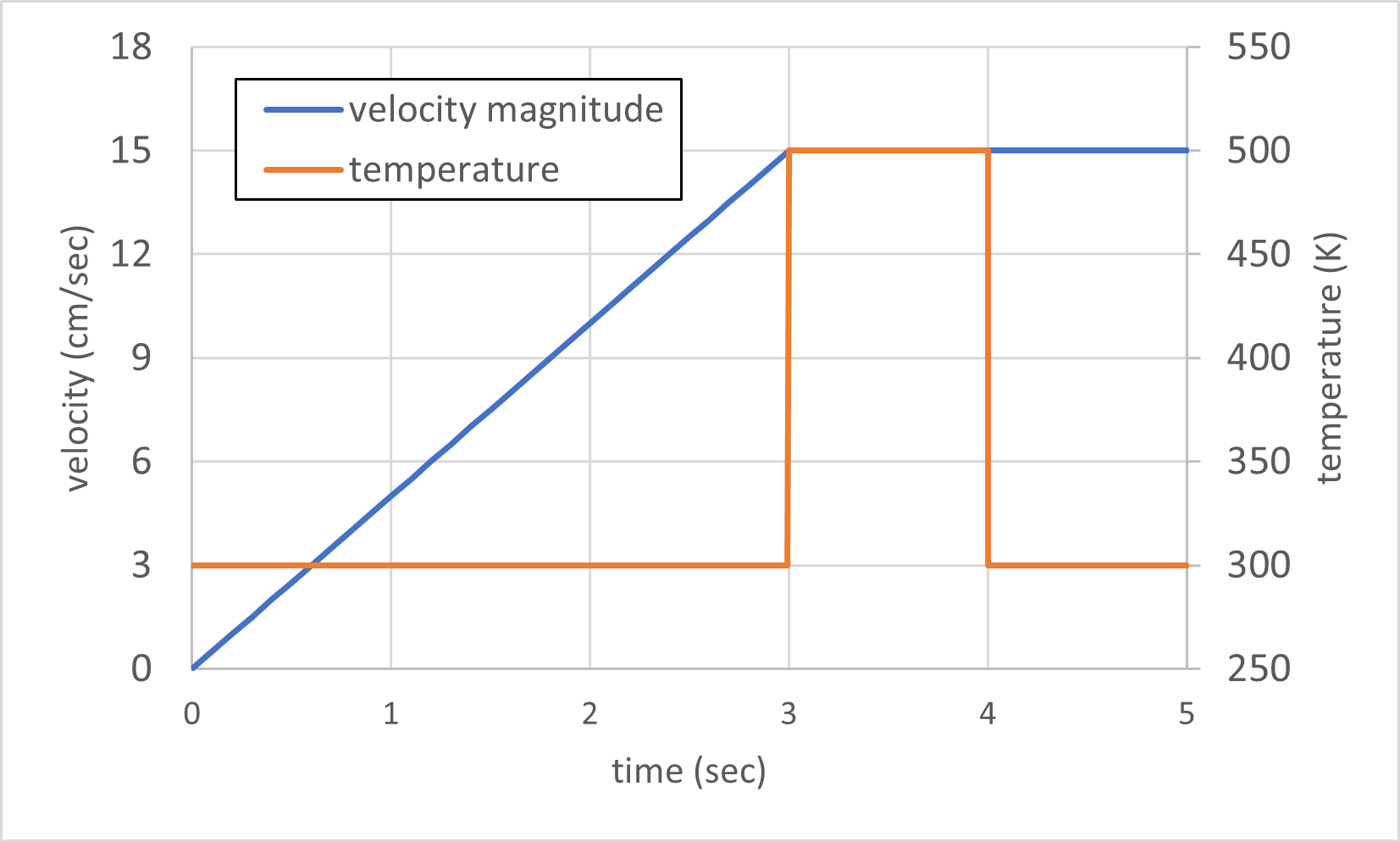
Fig. 9 Linear velocity ramp to 15 cm/s (0–3 s), constant thereafter; temperature step from 300 K to 500 K (3–4 s) then return to 300 K

Thermal boundary conditions

Boundary conditions can be applied to embedded boundaries (EBs). For example, a constant wall temperature can be imposed on the entire EB or restricted to a specific region.

To apply a boundary condition to only a portion of an EB, a face normal vector and tolerance can be specified. This allows the condition to be applied only to EB faces whose normals align with the specified direction within a given angular tolerance. The following inputs are defined using the prefix bc.[region_name].eb:

	Description	Type	Default
normal	[Optional] Specifies the target face normal direction. Only EB faces whose normals are parallel (within the specified tolerance) will have the boundary condition applied.	Reals<3>	None
normal_tol	[Optional] Angular tolerance (in degrees) used with eb.normal to select EB faces. A value of 0 requires exact alignment.	Real	0

The following table lists the thermal boundary condition options that can be applied to embedded boundaries (EBs), with inputs defined using the prefix bc.[region_name].eb.

	Description	Type	Default
temperature	Specify a wall temperature model for the embedded boundary. Options: adiabatic - no heat flux through the wall constant - impose a constant temperature along the EB. CHT-1D - compute a temperature for the wall using the 1D conjugate heat transfer model.	String	adiabatic
temperature.constant	Constant wall temperature. A valid is required for constant EB temperature model.	Real	None

The conjugate heat transfer model approximates heat transfer through the embedded boundary using a one-dimensional thermal resistance representation. By default, the wall temperature is computed from an algebraic heat balance; optionally, a lumped-capacity transient wall model can be enabled.

The external environment is treated as a thermal reservoir with constant temperature \(T_{\infty}\). Heat is transferred from the fluid to the inner wall surface, through the wall, and then from the outer wall surface to the environment, as illustrated in Fig. 10.

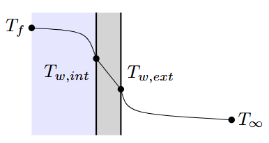
Fig. 10 Schematic of the conjugate heat transfer boundary condition.

The effective outward thermal conductance per unit area is

\[G_{out} = \left( \frac{L_w}{\kappa_w} + \frac{1}{h_{ext}} \right)^{-1}\]

where \(L_w\) is the wall thickness, \(\kappa_w\) is the wall thermal conductivity, and \(h_{ext}\) is the external convective heat transfer coefficient. This expression represents the combined resistance of conduction through the wall and convection from the outer wall surface to the environment.

For the zero-capacity wall model, the inner wall temperature is determined from an algebraic heat balance between internal convection, radiation, and heat transfer to the environment:

\[T_{w,int} = \frac{ h_{int} T_f - q_{rad} + G_{out} T_{\infty}}{h_{int} + G_{out}}\]

where \(h_{int}\) is the internal convective heat transfer coefficient. Positive \(q_{rad}\) denotes radiative heat loss from the wall. By default, the CHT-1D wall has no thermal storage, so the wall temperature responds instantaneously to changes in the local heat balance.

If a wall heat capacity \(C_A\) [J/(m²K)] is specified, the wall is modeled as a lumped thermal mass with a single spatially uniform temperature. In that case, the wall temperature evolves according to

\[C_A \frac{dT_{w,int}}{dt} = h_{int} \left( T_f - T_{w,int} \right) - q_{rad} - G_{out} \left( T_{w,int} - T_{\infty} \right)\]

In this lumped-capacity approximation, the inner and outer wall temperatures are not resolved separately; instead, the wall is represented by a single transient temperature. When \(C_A = 0\) or is not specified, the algebraic wall temperature model is used.

The model settings are defined using the prefix bc.[region_name].eb.temperature.CHT-1D:

	Description	Type	Default
T_env	Environment temperature	Real	None
h_int	Heat Transfer Coefficient (fluid–wall, internal) Specifies the convective heat transfer coefficient [W/m² K] between the fluid and adjacent solid walls (EBs) located within the interior of the computational domain.	Real	None
h_ext	Heat Transfer Coefficient (wall-environment, external) Specifies the convective heat transfer coefficient [W/m² K] between the wall and the external environment.	Real	None
wall.conductivity	The thermal conductivity of the wall.	Real	None
wall.thickness	Wall thickness.	Real	None
wall.heat_capacity	Lumped wall heat capacity per area [J/(m2K)]	Real
phase_averaged_temperature	Use a phase averaged temperature for simulations containing particles. The phase averaged temperature is computed as the volume fraction weighted sum of the fluid and averaged particle temperatures. \(T = \varepsilon_f T_f + (1-\varepsilon_f) \overline{T}_p\) The averaged particle temperature is computed by depositing the volume-averaged particle temperature to the grid. \(\overline{T}_p = \left( {\sum_p^{N_p} T_p V_p} \right) / \left( {\sum_p^{N_p} V_p} \right)\)	Bool	false

Below is an example for specifying a constant temperature boundary condition in the hot-walls region.

bc.regions = hot-walls

bc.hot-walls = eb
bc.hot-walls.eb.temperature = constant
bc.hot-walls.eb.temperature.constant = 800