Model options

The following inputs are defined using the mfix prefix.

	Description	Type	Default
gravity	Gravity vector [required]	Reals	0 0 0
advect_density	Flag to enable time evolution of fluid density.	int	0
advect_enthalpy	Flag to enable time evolution of fluid temperature and enthalpy.	int	0
solve_species	Flag to enable the time evolution of fluid species mass fractions.	int	0
constraint	Select low Mach number constraint. IncompressibleFluid constraint is appropriate for cold flow systems that do not have chemical reactions. Fluid temperature and species mass fractions act as passive tracers if advected. IdealGasOpenSystem constraint is used if the physical domain contains at least one pressure outflow boundary condition. The specified outflow (ambient) pressure is maintained so that the thermodynamic pressure is constant. IdealGasClosedSystem constraint is used for systems that are fully periodic or completely closed with no inflow / outflow boundaries. The thermodynamic pressure evolves in time to balance processes like chemical reactions.	string	IncompressibleFluid

Note

The thermodynamic pressure is a scalar value, not a scalar field. This is a consequence of the low Mach number assumption.

Fluid discretization

The following inputs are defined using the mfix prefix.

Key	Description	Type	Default
advection_type	Advection scheme mol Predictor-Corrector Method of Lines. MAC velocities and edge states are extrapolated in space. godunov Godunov. MAC velocities and edge states are extrapolated in space and time using a second-order Taylor series expansion.	string	Godunov
redistribution_type	Algorithms to address the ‘small cell problem’ associated with explicit cut-cell algorithms. StateRedist [BG21, GAB+22] FluxRedist [CC87, CGKM06] NoRedist: Do not redistribute fluxes.	String	StateRedist
redistribute_before_nodal_proj	Redistribute the velocity field before the nodal projection	Bool	True
redistribute_nodal_proj	Redistribute the velocity field after the nodal projection	Bool	False
use_drag_coeff_in_proj_gp	Algebraically consistent p coeff in proj or (default) simplified form	Bool	False
use_drag_in_godunov	Include a drag term in the Godunov flux or (default) not	Bool	False
godunov_ppm	When using Godunov, use piecewise parabolic (PPM) instead of piecewise linear (PLM) reconstruction	Bool	False
godunov_include_diff_in_forcing	When using Godunov, include viscous/diffusive terms in forcing terms	Bool	True
godunov_use_forces_in_trans	When using Godunov, add forcing terms in the construction of trans velocities	Bool	False
use_mac_phi_in_godunov	When using Godunov, don’t include the pressure gradient in the forcing term passed into the godunov routine; instead use gradient of mac phi which contains the full pressure	Bool	False
correction_small_volfrac	Threshold volume fraction for correcting small cell velocity at the end of the predictor and corrector	Real	1.e-4

Additional available constraints

Additional constraints may be imposed on problems which are under-determined such as particle settling in a fully periodic domain. Currently, only particle constraints are supported.

The following inputs are defined using the particles prefix.

	Description	Type	Default
constraint	Constraint type. Available options include: ‘mean_velocity’	String	None

For the mean_velocity constraint, the following inputs can be defined.

	Description	Type	Default
mean_velocity_x	mean particle velocity in dir=0	Real	Undefined
mean_velocity_y	mean particle velocity in dir=1	Real	Undefined
mean_velocity_z	mean particle velocity in dir=2	Real	Undefined

Below is an example for zero mean particle velocity in all three directions.

particles.constraint = "mean_velocity"

particles.constraint.mean_velocity_x = 0.
particles.constraint.mean_velocity_y = 0.
particles.constraint.mean_velocity_z = 0.

In the above example, at the end of each (fluid) time step, the global mean particle velocity is computed in each direction, then subtracted from each particle’s velocity vector so that the mean particle velocity for the system is zero.

Deposition scheme

The following inputs are defined using the mfix prefix.

	Description	Type	Default
deposition_scheme	The algorithm used to transfer particle properties to the Eulerian grid. An overview of the schemes is provided below. centroid trilinear true-dpvm trilinear-dpvm-square	String	trilinear
deposition_scale_factor	The deposition scale factor. Applicable only with true-dpvm and trilinear-dpvm-square deposition schemes. The value must be in the intervarl \([0,\Delta x/2]\) where \(\Delta x\) is the mesh spacing.	Real	1.0
deposition_diffusion_coeff	If a positive value is set, a diffusion equation with this diffusion coefficient is solved to smooth deposited quantities.	Real	-1.0

In the following subsections, the four deposition methods are briefly described and illustrated.

Centroid

The centroid deposition scheme transfers particle properties, for example volume, to the Eulerian grid cell containing its center. Illustrated in two-dimensions below, the particle center is in the upper-right cell; therefore, the deposition weight for that cell is 1 and all other weights are zero.

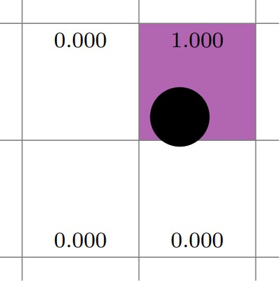
Fig. 5 Example of centroid deposition.

Trilinear

Trilinear deposition transfers particle properties to the eight Eulerian grid cells surrounding its center. First, low and high weights are calculated for each direction, then they are multiplied together to form eight composite weights. The following figure illustrates bilinear interpolation. The left image shows weights computed in the X-direction, \([0.15, 0.85]\), and the center image shows weights computed in the Y-direction, \([0.25,0.75]\). The right image shows the composite weights for the four cells that comprise the 2D neighborhood surrounding the particle.

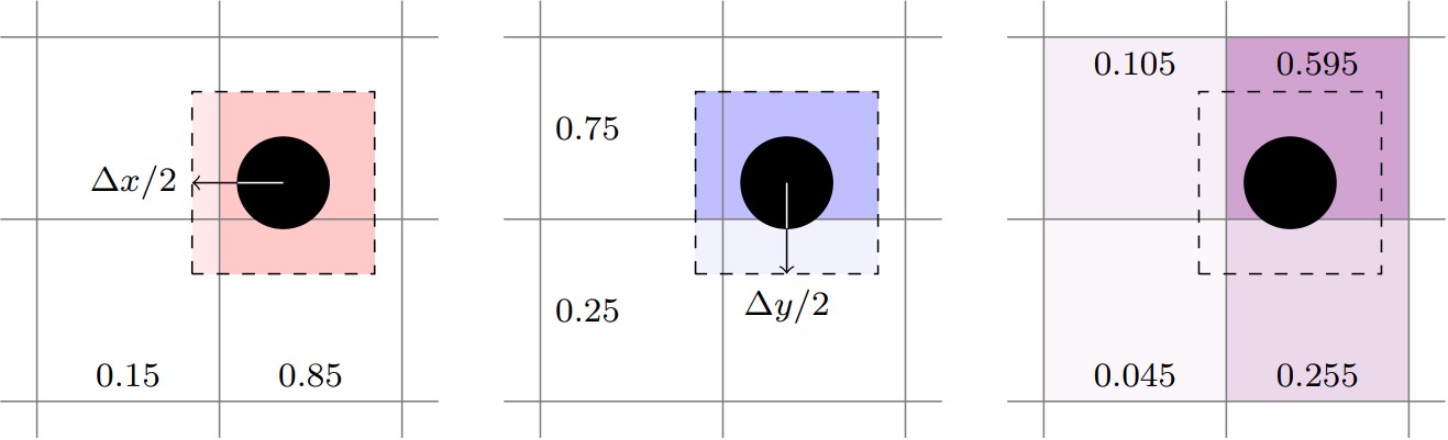
Fig. 6 Example of trilinear deposition.

True-DPVM

The “true” divided particle volume method (DPVM) calculates the actual volume of a particle in each cell by computing the intersection between the grid cell faces and the particle. The fractional volume (volume inside the cell divided by total particle volume) is used as the deposition weight. If the deposition_scale_factor is defined, it multiplies the particle radius increasing the effective area to transfer properties over. The true-DPVM scheme is illustrated below where the dashed line represents the scaled particle radius. The grown particle intersects the top two and lower-right cells. Since the grown particle does not intersect the lower-left cell, it has a deposition weight of zero.

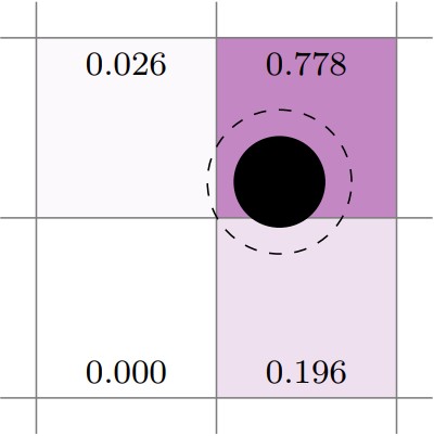
Fig. 7 Example of true-dpvm deposition.

Trilinear DPVM square

The trilinear DPVM square method is similar to the trilinear scheme in that low and high weights are computed for each direction, then multiplied together to give a composite weight for each of the eight cells in the neighborhood. The primary distinction is that the fractional volume cut by the grid cell face for each direction is used to calculate the low and high weights. If the deposition_scale_factor is defined, it multiplies the particle radius increasing the effective area to transfer properties over. In the below figure, the left image shows the X-direction weights, and the center image shows the Y-direction weights. The right image shows the resulting composite weights.

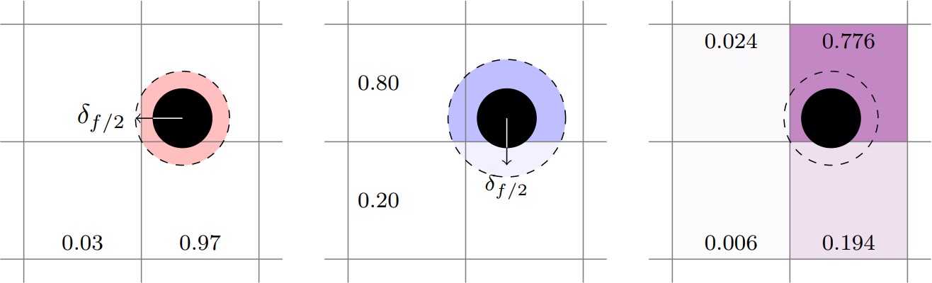
Fig. 8 Example of trilinear dpvm square deposition.

Deposition redistribution

The following inputs are defined using the mfix prefix.

Key	Description	Type	Default
deposition_redist_type	Algorithm used to redistribute excess solids to adjacent cells. This typically applies only to small cut-cells along the geometry. MaxPack If the solids volume fraction exceeds the prescribed max_solids_volume_fraction, then the local average solids volume is computed and solids volume exceeding the average is reallocated to adjacent cells. The fraction of redistributed solids is applied to all transferred properties. StateRedist Use the state redistribution algorithm of [BG21, GAB+22] to reallocate transferred quantities in small cells.	String	MaxPack
max_solids_volume_fraction	Threshold solids volume fraction for MaxPack redistribution. Redistribution of transferred quantities only occurs when the solids volume fraction of a cell exceeds this value.	Real	0.6
deposition_redist_vfrac	Threshold geometric volume fraction StateRedist redistribution. Redistribution of transferred quantities always occurs for cells with a geometric volume fraction below this value.	Real	0.1

Fluid-particle drag

The following input is defined using the mfix.drag prefix.

	Description	Type	Default
model	Fluid-particle drag model. WenYu [WY66] Gidaspow [DG90, LB00] BVK2 [BvdHK07a, BvdHK07b, TPK+15, TGS11] SyamOBrien [SOBrien88] UserDrag	String	None
model.SyamOBrien.c1 model.SyamOBrien.d1	Fitting parameters for SyamOBrien drag model	Real	None
include_divtau	Interpolate the fluid shear stress to particles and include in the fluid-particle drag force. The force is applied to the fluid by multiplying the shear stress by fluid volume fraction.	int	0
virtual_mass	Include virtual mass force in fluid-particle momentum transfer. The virtual mass force is not included by default. \(\mathbf{F}_p^{vm} = -C_p^{vm}\rho_f \left( \frac{D\mathbf{u}_f}{Dt} - \frac{d\mathbf{u}_p}{dt}\right)\mathcal{V}_p\) Null zero virtual mass coefficient, \(C_p^{vm}=0\) Constant - user-specified constant coefficient Zuber [Zub64] \(C_p^{vm} = \frac{1}{2}\frac{1+2\varepsilon_p}{1-\varepsilon_p}\) Nijssen [NKvandStel+20] \(\begin{split}C_p^{vm} =& C_0^{vm} \\ &+ \sum_{k=1}^3\left\{ \left[ a_{k,0} + a_{k,1} \ln \left( \frac{\rho_p}{\rho_f} \right) \right] \varepsilon_p^k \right\}\end{split}\)	String	None
virtual_mass.constant	Constant virtual-mass coefficient.	Real	0.5

Note

The UserDrag keyword is used to invoke a user defined drag model. This is accomplished by copying src/usr/usr_drag.cpp file into the build directory, implementing the desired drag model, and recompiling the code. An example can be found in tests/DEM06-x.

Heat transfer coefficients

The following input is defined using the mfix.convection prefix.

	Description	Type	Default
model	Fluid-particle heat transfer coefficient model. RanzMarshall [RM52] Gunn [Gun78] NullConvection - disable fluid-particle heat transfer	String	RanzMarshall