2.5. MMS01: Single-phase, 2D, sinusoidal functions¶
2.5.1. Description¶
A sinusoidal divergence-free manufactured solution [12, 13] for the fluid pressure, \(P_{g}\), and \(x\) and \(y\) velocity components, \(u_{g}\) and \(v_{g}\), respectively, is used for the verification of steady-state, single-phase flows on a 2D grid.
Fig. 2.7 shows a color contour of the pressure field and velocity streamlines for the manufactured solution using constants \(P_{g0} = 100\ \text{Pa}\), \(u_{g0} = 5.0\ \mathrm{m \cdot sec}^{- 1}\), and , \(v_{g0} = 5.0\mathrm{\ m \cdot sec}^{- 1}\).
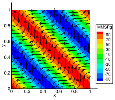
Fig. 2.7 Pressure contours and velocity streamlines for 2D, single-phase, simple sinusoidal manufactured solution on a 64x64 cell grid.¶
2.5.2. Setup¶
Computational/Physical model |
||
|---|---|---|
2D, Steady-state, incompressible |
||
Single-phase (no solids) |
||
No gravity |
||
Thermal energy equation is not solved |
||
Turbulence equations are not solved (Laminar) |
||
Uniform mesh |
||
Superbee and Central discretization schemes |
||
Geometry |
||
Coordinate system |
Cartesian |
|
x-length |
1.0 |
(m) |
y-length |
1.0 |
(m) |
Material † |
||
Fluid density, \(\rho_{g}\) |
1.0 |
(kg·m-3) |
Fluid viscosity, \(\mu_{g}\) |
1.0 |
(Pa·s) |
Initial Conditions |
||
Pressure (gauge), \(P_{g}\) |
0.0 |
(Pa) |
x-velocity, \(u_{g}\) |
5.0 |
(m·s-1) |
y-velocity, \(v_{g}\) |
5.0 |
(m·s-1) |
Boundary Conditions ‡ |
||
All boundaries |
Mass inflow |
† Material properties selected to ensure comparable contribution from convection and diffusion terms.
‡ The manufactured solution is imposed on all boundaries (i.e., Dirichlet specification).
2.5.3. Results¶
Numerical solutions were obtained using both Superbee and Central discretization schemes for 8x8, 16x16, 32x32, 64x64, and 128x128 grid meshes. The Superbee scheme order of accuracy tests show a first-order rate of convergence for pressure under the \(L_{\infty}\ \)norm as illustrated in Fig. 2.8 (a), whereas the formal order for this scheme is two. The largest errors in pressure are local to boundary cells along the West (y=0) and South (x=0) edges of the domain as shown in Fig. 2.9 (a). This is an artifact of the staggered grid implementation in MFIX where only a single ghost cell layer is present along West and South boundaries, reducing higher-order upwind schemes to first-order. This effect also occurs along the Bottom (z=0) edge of the domain for three-dimensional simulations. Further investigation is needed to determine to what extent the errors introduced at the boundary propagate into the domain interior.
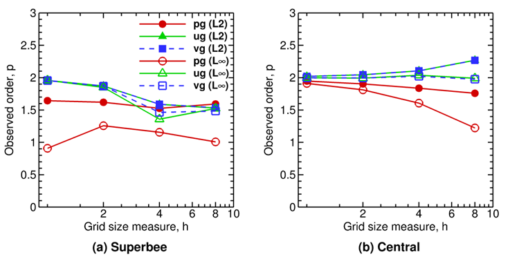
Fig. 2.8 Observed orders of accuracy for 2D, single-phase, sinusoidal manufactured solution. (a) Superbee scheme, (b) Central scheme.¶
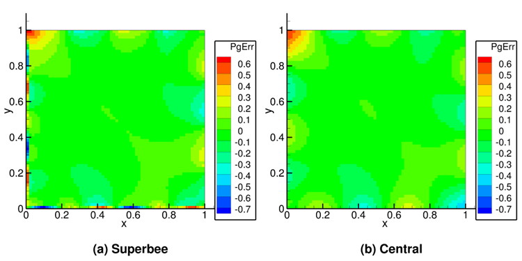
Fig. 2.9 Errors in pressure for 2D, single-phase, sinusoidal manufactured solution for grid resolution (64x64). (a) Superbee scheme, (b) Central scheme¶
The Central scheme results, depicted in Fig. 2.8 (b), show second order accuracy for all variables. The formal order for the Central scheme is recovered because no up-winding is performed, thereby averting solution deterioration at the boundaries. The errors in pressure near the boundaries are consistent with the scheme’s formal order as can be seen from Fig. 2.9 (b).
2.5.4. Notes¶
During initial testing, it was discovered that the strain-tensor cross terms for the momentum equations were not calculated within steady-state sub-iterations which lead to large errors (not shown). These errors do not appear in cases with zero shear at the boundaries. Transient simulations recalculate these cross-terms at the start of each time-step making it difficult to determine the effect on the solution. The significance of this simplification (likely done to reduce computational expense) on real-world application problems is unknown and should be investigated. For MMS tests, this issue was circumvented by recalculating the cross-terms of the strain-tensor at each sub-iteration.