2.6. MMS02: Two-phase, 3D, curl-based functions with constant volume fraction

2.6.1. Description

Assuming that gas and solid volume fractions (i.e., \(\varepsilon_{g}\) and \(\varepsilon_{s}\)) remain constant, we can see from gas and solid continuity equations that both fluid and solid velocity fields are divergence-free (for constant density of fluid and solids). A manufactured solution for the fluid-phase velocity field is defined using the curl-based approach developed in [5]. For the solid-phase velocity field, a set of simple sinusoidal functions is selected (same as those shown in Eq.2.45). The manufactured solutions for scalar quantities (pressure, gas temperature, and solid temperature) can be multivariate functions of sines and cosines as defined in Eq.6.1. The selected functions for all concerned variables are shown over a 3D domain in Fig. 2.10 through Fig. 2.12.

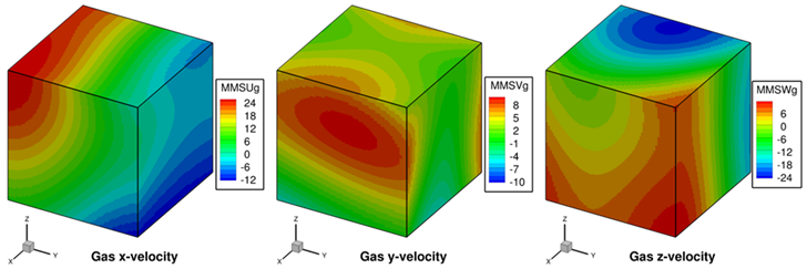
Fig. 2.10 Gas phase momentum equation manufactured solutions for 3D, steady-state, two-phase flow verification test case.

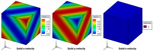
Fig. 2.11 Solids phase momentum equation manufactured solutions for 3D, steady-state, two-phase flow verification test case.

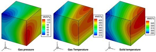
Fig. 2.12 Scalar field manufactured solutions for 3D, steady-state, two-phase flow verification test case.

2.6.2. Setup

Table 2.14 MMS-02 Setup, Initial and Boundary Conditions.

Computational/Physical model
3D, Steady-state, incompressible
Two-phase
No gravity
Drag model is turned off
Friction model is turned off
Thermal energy equations are solved
Granular energy equation is not solved
Turbulence equations are not solved (Laminar)
Central scheme
Geometry
Coordinate system	Cartesian
Domain length, \(L\) (x)	1.0	(m)
Domain height, \(H\) (y)	1.0	(m)
Domain width, \(W\) (z)	1.0	(m)
Material †
Fluid density, \(\rho_{g}\)	1.0	(kg·m-3)
Fluid viscosity, \(\mu_{g}\)	1.0	(Pa·s)
Fluid specific heat, \(C_{\text{pg}}\)	0.05	(J·kg-1·K-1)
Fluid thermal conductivity, \(k_{g}\)	1.0	(J·kg-1·K-1·s-1)
Solids density, \(\rho_{s}\)	2.0	(kg·m-3)
Solids viscosity, \(\mu_{s}\)	2.0	(Pa·s)
Solids specific heat, \(C_{\text{ps}}\)	0.1	(J·kg-1·K-1)
Solids thermal conductivity, \(k_{s}\)	2.0	(J·kg-1·K-1·s-1)
Initial Conditions
Pressure (gauge), \(P_{g}\)	0.0	(Pa)
Fluid x-velocity, \(u_{g}\)	10.0	(m·s-1)
Fluid y-velocity, \(v_{g}\)	10.0	(m·s-1)
Fluid z-velocity, \(w_{g}\)	10.0	(m·s-1)
Solids x-velocity, \(u_{s}\)	5.0	(m·s-1)
Solids y-velocity, \(v_{s}\)	5.0	(m·s-1)
Solids z-velocity, \(w_{s}\)	5.0	(m·s-1)
Fluid temperature, \(T_{g}\)	350.0	(K)
Solids temperature, \(T_{s}\)	300.0	(K)
Gas volume fraction, \(\varepsilon_{g}\)	0.7	–
Boundary Conditions ‡
All boundaries	Mass inflow

† Material properties selected to ensure comparable contribution from convection and diffusion terms. Specified values are constant to avoid the introduction of constitutive laws.

^‡ The manufactured solution is imposed on all boundaries (i.e., Dirichlet specification).

2.6.3. Results

Numerical solutions were obtained using the Central discretization scheme for 8x8, 16x16, 32x32, 64x64, and 128x128 grid meshes. The observed order approaches second order for both \(L_{2}\) and \(L_{\infty}\) norms using the Central scheme, as shown in Fig. 2.13. This indicates that the numerical discretization terms have been implemented correctly for all derivative terms within the gas momentum equations, solid momentum equations, gas pressure correction equation, gas energy equation, and solid energy equation.

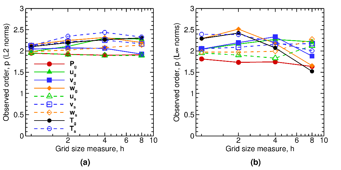
Fig. 2.13 Observed orders of accuracy for 3D, two-phase flows (constant volume fraction) using (a) \(\mathbf{L}_{\mathbf{2}}\) norms, and (b) \(\mathbf{L}_{\mathbf{\infty}}\) norms of the discretization error.