2.3. MMS-EX02: One dimensional steady state heat equation

2.3.1. Description

The gas phase energy equations in MFIX are:

(2.25)\[\varepsilon_{g}\rho_{g}{C_{p}}_{g}\left\lbrack \frac{\partial T_{g}}{\partial t} + U_{\text{gj}}\frac{\partial T_{g}}{\partial x_{j}} \right\rbrack = - \frac{\partial}{\partial x_{j}}\left( - \varepsilon_{g}\kappa_{g}\frac{\partial T_{g}}{\partial x_{j}} \right) - \sum_{n = 1}^{N_{g}}{h_{\text{gn}}R_{\text{gn}}} + \mathcal{S}_{g}\]

The energy equations can be recast as the one-dimensional heat equation by imposing the following simplifying assumptions: 3

1. A steady state simulation is needed to remove the energy equations’ transient term.

2. Calculations are restricted to one dimension.

3. The domain length in the x-axial direction is \(\text{xϵ}\left\lbrack 0,5 \right\rbrack\).

4. The gas volume fraction, density, thermal conductivity, and specific heat are set to one,

   \(\varepsilon_{g} = 1\), \(\rho_{g} = 1\), \(\kappa_{g} = 1\), and \(C_{\text{pg}} = 1\).

5. The gas momentum equations are not solved and initial velocity field is set to zero so that the convective term is zero.

6. There are no chemical reactions, interphase mass transfer or other sources of energy implying: \(\sum_{n = 1}^{N_{g}}{h_{\text{gn}}R_{\text{gn}}} + \mathcal{S}_{g} = 0\).

On re-evaluation of the energy equations, the following one-dimensional form (aka the steady state heat equation) emerges:

(2.26)\[\frac{\partial^{2}T_{g}}{\partial x^{2}} = 0\]

Following the method of manufactured solutions, the partial differential equation is recast as:

(2.27)\[L\left( x \right) = \left( T_{g} \right)_{\text{xx}} = 0\]

MMS requires the selection of a manufactured solution. Because this is a steady-state form, the manufactured solution is chosen not to incorporate a time variable for simplicity. Arbitrarily, choose any suitable analytic form of appropriate continuous, differential order. In this case, observe that whatever manufactured solution we choose must be continuously differentiable through its second spatial derivative. Also note, in MFIX, temperature is calculated absolutely and is restricted as: \(250 < u < 4000\ \)(which represents the Kelvin scale). Values outside of these bounds cause a fatal error within the code. So, in this case, there is a caveat that requires the manufactured solution chosen cannot present out-of-bound values on any domain of interest. In this example, the domain,\(\ 0 \leq x \leq 5\), and the manufactured solution:

(2.28)\[T_{g}\left( x \right) = 500 + \left( 1 + x^{3} \right) = 501 + \ x^{3}\]

work within the MFIX constraints. Continuing to follow the MMS, this solution is applied to \(L\left( x \right)\):

(2.29)\[L{(x)}_{T_{g}(x)} = \frac{\partial^{2}}{\partial x^{2}}\left( 501 + \ x^{3} \right)\]

(2.30)\[L{(x)}_{T_{g}(x)} = 6x\]

Then, appropriate initial and/or boundary conditions are cast. For this case, since time is inconsequential, no initial condition is warranted. Focus then shifts to boundary conditions.

On the domain of interest: \(\text{xϵ}\left\lbrack 0,5 \right\rbrack\), Dirichlet boundary conditions are:

(2.31)\[\begin{split}\begin{matrix} T_{g}\left( 0 \right) = 501 + 0^{3} = 501 \\ T_{g}\left( 5 \right) = 501 + 5^{3} = 501 + 125 = 626 \\ \end{matrix}\end{split}\]

2.3.2. Setup

This case is designed to test the energy equation implementation.

Table 2.4 MMS-EX02 Setup, Initial and Boundary Conditions.

Computational/Physical model
1D, Steady-state, incompressible
Single-phase (no solids)
No gravity
Turbulence equations are not solved (Laminar)
Uniform mesh
Central scheme
Geometry
Coordinate system	Cartesian
Domain length, \(L\) (x)	5.0
Material †
Fluid density, \(\rho_{g}\)	1.0	(kg·m-3)
Fluid viscosity, \(\mu_{g}\)	1.0	(Pa·s)
Fluid specific heat, \(C_{pg}\)	1.0	(J·kg-1·K-1)
Initial Conditions
Pressure (gauge), \(P_{g}\)	0.0	(Pa)
Temperature, \(T_{g}\)	550.0
Boundary Conditions ‡
East/West (x)	(MMS)
All other boundaries	Adiabatic Walls

† Material properties selected to ensure comparable contribution from convection and diffusion terms.

^‡ The manufactured solution imposed on the east / west boundaries is given by Eq.2.31.

User defined functions specific to the MMS implementation in MFIX are used to introduce the source term. Specifically, for each computational cell, Eq.2.30 is evaluated and subtracted from the right hand side of the linear equation. Once the simulation has converged, the \(L_{1}\), \(L_{2}\) and \(L_{\infty}\) error norms are computed by referencing Eq.2.28.

2.3.3. Results

Following the outline of MMS methodology, three separate 1-dimensional systems (x, y and z) were created, each having 8, 16, 32, 64, 128, and 256 cells, using the steady state heat equation and manufactured solution previously described.

An observed order for each direction is calculated using \(L_{1}\), \(L_{2}\) and \(L_{\infty}\) error norms. The following tables and figure illustrate these data. One can quickly see from the tabled L-norms and subsequently calculated observed order that direction does not have a large influence on these values. All data points to a 2^nd order (p) convergence of the steady state heat equation using MFIX.

Hence, these data imply that the diffusion term engaged in the energy equation through the evaluation of the steady state heat equation is numerically closed on 2^nd order approximations which is correct and verified by the method of manufactured solutions.

Table 2.5 Observed Order, p, for steady state heat equation using \(\mathbf{U}\left( \mathbf{x} \right)\mathbf{= 501 + \ }\mathbf{x}^{\mathbf{3}}\) on \(\mathbf{0 \leq x \leq 5}\).

Mesh	L 1-norm	L 2-norm	L ∞-norm	p (L 1)	p (L 2)	p (L ∞)
8	7.3242E-01	8.4407E-01	1.3733E+00	N/A	N/A	N/A
16	1.8311E-01	2.1133E-01	3.5477E-01	2.0000	1.9979	1.9527
32	4.5776E-02	5.2852E-02	9.0122E-02	2.0000	1.9995	1.9769
64	1.1444E-02	1.3214E-02	2.2709E-02	2.0000	1.9999	1.9886
128	2.8610E-03	3.3036E-03	5.6997E-03	2.0000	2.0000	1.9943
256	7.1525E-04	8.2590E-04	1.4277E-03	2.0000	2.0000	1.9972

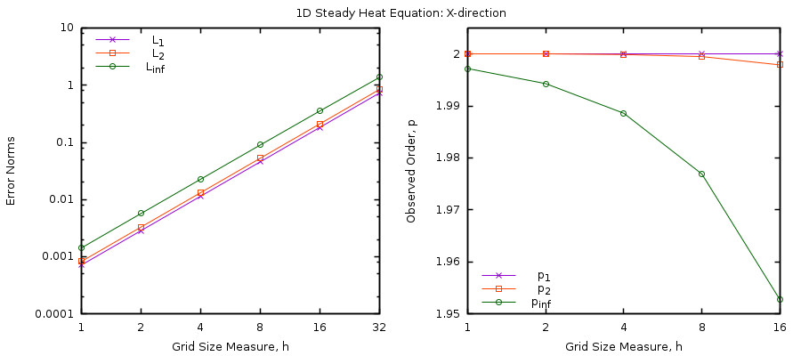
Fig. 2.3 Observed Order, MMS Solution to 1-D steady state heat equation in MFIX, using \(\mathbf{U}\left( \mathbf{x} \right)\mathbf{= 501 + \ }\mathbf{x}^{\mathbf{3}}\) on \(\mathbf{0 \leq x \leq 5}\).

3

Again, simplifying assumptions are typically avoided when using the MMS. However, this example intentionally simplifies the energy equations to make the example easier to follow.