2.2. MMS-EX01: One dimensional steady state Burger’s equation¶
2.2.1. Description¶
The gas-phase momentum equations in MFIX have the following generalized form: 1
where,
To build on the previous example, the momentum equations can be recast as the one-dimensional steady state Burger’s equation by imposing the following simplifying assumptions: 2
A steady state simulation is needed to remove the momentum equations’ transient term.
Calculations are restricted to one dimension.
The domain is of unit length in the x-axial direction: \(\text{xϵ}\left\lbrack 0,5 \right\rbrack\).
The gas volume fraction and density are set to one, \(\varepsilon_{g} = 1\) and \(\rho_{g} = 1\).
The gas viscosity is chosen as \(\mu_{g} = 3/4\).
Gravity and all other source terms are set to zero, \(g = 0\) and \(\mathcal{S}_{\text{gi}} = 0\).
Finally, because the pressure solver is integrated with the momentum equations, it is important to decouple the pressure correction step from the calculation.
The momentum equations with the above simplifications reduce to the one-dimensional Burger’s equation,
where the subscript indicating dimensionality has been dropped for notational clarity.
Following the method of manufactured solutions, the partial differential equation is recast as:
MMS requires the selection of a manufactured solution. Arbitrarily, choose any suitable analytic form of appropriate continuous, differential order. In this case, note that whatever manufactured solution is chosen must be continuously differentiable through its second derivative. Aside from asymptotic functions that may exhibit unphysical local changes, most any analytic function will be a suitable choice for this application. So, keeping things simple, as in the prior explanation,
Then, apply this form to \(L\left( x \right)\):
Finally, cast appropriate initial and/or boundary conditions. For this case, since time is inconsequential, no initial condition is warranted. Focus then shifts to boundary conditions. With the domain of interest being \(\text{xϵ}\left\lbrack 0,1 \right\rbrack\), fixed boundary conditions are given by:
(2.24)¶\[\begin{split}\begin{matrix} U\left( 0 \right) = 0.5 + \sin\left( 0 \right) = 0.5 \\ U\left( 1 \right) = 0.5 + sin(5) \\ \end{matrix}\end{split}\]
2.2.2. Setup¶
Initially, only the x-direction momentum equation on a domain with unit dimensions is considered. Subsequently, the setup is executed in the y- and z- directions to determine if problem orientation influences the observed order.
Computational/Physical model |
||
|---|---|---|
1D, Steady-state, incompressible |
||
Single-phase (no solids) |
||
No gravity |
||
Turbulence equations are not solved (Laminar) |
||
Uniform mesh |
||
Central scheme |
||
Geometry |
||
Coordinate system |
Cartesian |
|
Domain length, \(L\) (x) |
1.0 |
|
Material † |
||
Fluid density, \(\rho_{g}\) |
1.0 |
(kg·m-3) |
Fluid viscosity, \(\mu_{g}\) |
0.75 |
(Pa·s) |
Initial Conditions |
||
Pressure (gauge), \(P_{g}\) |
0.0 |
(Pa) |
Fluid x-velocity, \(u_{g}\) |
1.0 |
(m·sec-1) |
Boundary Conditions ‡ |
||
East/West (x) |
Mass inflow (MMS) |
|
All other boundaries |
Cyclic |
† Material properties selected to ensure comparable contribution from convection and diffusion terms.
‡ The manufactured solution imposed on the east / west boundaries is given by Eq.2.24.
User-defined functions specific to the MMS implementation in MFIX are used to introduce the source term. Specifically, for each discretized x-momentum computational cell, equation Eq.2.23 is evaluated and subtracted from the right hand side of the linear equation. Once the simulation has converged, the \(L_{1}\), \(L_{2}\) and \(L_{\infty}\) error norms are computed by referencing equation Eq.2.24.
2.2.3. Results¶
Following the outline of MMS methodology, three separate 1-dimensional systems (x, y and z) were created, each having 4,8, 16, 32, 64, and 128 cells, using the steady state Burger’s equation and manufactured solution previously described.
An observed order for each direction is calculated using \(L_{1}\), \(L_{2}\) and \(L_{\infty}\) error norms. The following tables and figure illustrate these data. One can quickly see from the tabled L-norms and subsequently calculated observed order that direction does not have a large influence on these values. All data points to a 2nd order (p) convergence of the steady state Burger’s equation using MFIX. In the present input-deck construction, whereby the numerical method implemented is central differencing method, this is the best outcome to expect.
Mesh |
L 1-norm |
L 2-norm |
L ∞-norm |
p (L 1) |
p (L 2) |
p (L ∞) |
|---|---|---|---|---|---|---|
4 |
2.4834E-01 |
2.5853E-01 |
3.1909E-01 |
N/A |
N/A |
N/A |
8 |
5.2081E-02 |
5.3318E-02 |
7.0000E-02 |
2.2535 |
2.2776 |
2.1886 |
16 |
1.1771E-02 |
1.2317E-02 |
1.6652E-02 |
2.1455 |
2.1139 |
2.0716 |
32 |
2.8250E-03 |
2.9965E-03 |
4.1128E-03 |
2.0589 |
2.0393 |
2.0176 |
128 |
6.9383E-04 |
7.4135E-04 |
1.0251E-03 |
2.0256 |
2.0151 |
2.0043 |
Hence, these data imply that the terms engaged in the momentum equation through the evaluation of the steady state Burger’s equation are numerically closed on 2nd order approximations which is correct and verified by the method of manufactured solutions.
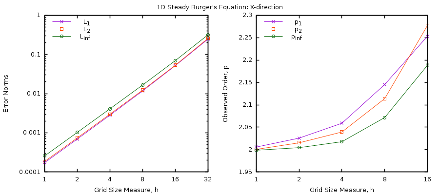
Fig. 2.2 Observed Order, MMS Solution to 1-D steady state Burger’s equation in MFIX, using \(\mathbf{U}\left( \mathbf{x} \right)\mathbf{= 1 +}\mathbf{sin}\mathbf{(x)}\) on \(\mathbf{0 \leq x \leq 1}\).¶
As a final observation, note that observed order appears to increase with decreasing spatial mesh. However, as expected, L-norms decrease with increasing mesh density, indicating a better overall solution.
- 1
The conservative form of the fluid momentum equations is presented here, however, the non-conservative form is solved in MFIX. The non-conservative form is obtained by subtracting the continuity equation from the conservative form.
- 2
Assumptions that reduce model complexity are typically avoided when using the MMS. However, this example intentionally simplifies the momentum equations to make the example easier to follow.