2.4. MMS-EX03: One dimensional transient heat equation¶

2.4.1. Description¶

Again consider the gas phase energy equations in MFIX given by equation (2‑25) in the previous example. The energy equations can be recast as the 1-dimensional transient heat equation by imposing the following simplifying assumptions:

Calculations are restricted to one dimension.
The domain length in the x-axial direction is \(\text{xϵ}\left\lbrack 0,1 \right\rbrack\).
The gas volume fraction, density, thermal conductivity, and specific heat are set to one,

\(\varepsilon_{g} = 1\), \(\rho_{g} = 1\), \(\kappa_{g} = 1\), and \(C_{\text{pg}} = 1\).
The gas momentum equations are not solved and initial velocity field is set to zero so that the convective term is zero.
There are no chemical reactions, interphase mass transfer or other sources of energy implying: \(\sum_{n = 1}^{N_{g}}{h_{\text{gn}}R_{\text{gn}}} + \mathcal{S}_{g} = 0\).

On re-evaluation of the energy equations, the following one-dimensional form (aka the transient heat equation) emerges:

(2.32)¶\[\frac{\partial T_{g}}{\partial t} - \frac{\partial^{2}T_{g}}{\partial x^{2}} = 0\]

Following the MMS approach, the partial differential equation is recast as:

(2.33)¶\[L\left( x,t \right) = \frac{\partial T_{g}}{\partial t} - \alpha\frac{\partial^{2}T_{g}}{\partial x^{2}} = 0\]

As MMS requires the selection of a manufactured solution, a suitable analytic form of appropriate continuous, differential order is chosen. In this case, note that whatever manufactured solution is picked must be continuously differentiable through its second spatial derivative and first temporal derivative. In addition, for illustrative purposes, the manufactured solution is chosen so that time will appear in the boundary conditions. For simplicity, MMS-EX02 is modified by incorporating a time value, t, as:

(2.34)¶\[T_{g}\left( x,t \right) = T_{g0} + T_{\text{gx}}\cos\left( A_{\text{Tgx}}\text{πx} \right) + T_{\text{gt}}\cos\left( A_{\text{Tgt}}\text{πt} \right) + T_{\text{gtx}}\cos\left( A_{\text{Tgtx}}\text{πtx} \right)\]

with a simple domain: \(\left\{ t \geq 0,\ \ \ 0 \leq x \leq 1 \right\}\).

Then, this form is applied to \(L\left( x,t \right)\):

(2.35)¶\[L{(x,t)}_{T_{g}(x,t)} = \frac{\partial}{\partial t}T_{g}\left( x,t \right) - \alpha\frac{\partial^{2}}{\partial x^{2}}T_{g}\left( x,t \right)\]

(2.36)¶\[\begin{split}L{(x,t)}_{T_{g}(x,t)} =& -T_{\text{gt}}\left( A_{\text{Tgt}}\pi \right)\sin\left( A_{\text{Tgt}}\text{πt} \right) - T_{\text{gxt}}\left( A_{\text{Tgtx}}\text{πx} \right)\sin\left( A_{\text{Tgtx}}\text{πtx} \right) \\ & + \alpha T_{\text{gx}}\left( A_{\text{Tgx}}\pi \right)^{2}\cos\left( A_{\text{Tgx}}\text{πx} \right) + \alpha T_{\text{gtx}}\left( A_{\text{Tgtx}}\pi \right)^{2}\cos\left( A_{\text{Tgtx}}\text{πtx} \right)\end{split}\]

Then, appropriate initial and/or boundary conditions are cast. For this case, an appropriate initial condition is:

(2.37)¶\[T_{g}\left( x,0 \right) = T_{g0} + T_{\text{gx}}\cos\left( A_{\text{Tgx}}\text{πx} \right) + T_{\text{gt}} + T_{\text{gtx}}\]

Focus then shifts to boundary conditions. On the spatial domain of interest: \(\text{xϵ}\left\lbrack 0,1 \right\rbrack\), boundary conditions become:

(2.38)¶\[\begin{split}\begin{matrix} T_{g}\left( 0,t \right) = T_{g0} + T_{\text{gx}} + T_{\text{gt}}\cos\left( A_{\text{Tgt}}\text{πt} \right) + T_{\text{gtx}} \\ T_{g}\left( 1,t \right) = T_{g0} + T_{\text{gx}}\cos\left( A_{\text{Tgx}}\pi \right) + T_{\text{gt}}\cos\left( A_{\text{Tgt}}\text{πt} \right) + T_{\text{gtx}}\cos\left( A_{\text{Tgtx}}\text{πt} \right) \\ \end{matrix}\end{split}\]

Note that these boundary conditions, while Dirichlet in nature, are dependent on time. The parameters chosen in the manufactured solution are summarized below:

Table 2‑4: Parameters used in MMS applied to transient heat conduction

Table 2.6 Parameters used in MMS applied to transient heat conduction¶
\(T_{g0}\)	500 K
\(T_{\text{gx}}\)	10 K
\(T_{\text{gt}}\)	100 K
\(T_{\text{gtx}}\)	10 K
\(A_{\text{Tgx}}\)	2.0
\(A_{\text{Tgt}}\)	2.0
\(A_{\text{Tgtx}}\)	2.0

2.4.2. Setup¶

This case is designed to test the energy equation implementation.

Table 2.7 MMS-EX03 Setup, Initial and Boundary Conditions.¶
Computational/Physical model
1D, Steady-state, incompressible
Single-phase (no solids)
No gravity
Turbulence equations are not solved (Laminar)
Uniform mesh
Central scheme

Geometry
Coordinate system	Cartesian
Domain length, \(L\) (x)	1.0	(m)

Material ^†
Fluid density, \(\rho_{g}\)	1.0	(kg·m^-3)
Fluid viscosity, \(\mu_{g}\)	1.0	(Pa·s)
Fluid specific heat, \(C_{pg}\)	1.0	(J·kg^-1·K^-1)

Initial Conditions
Pressure (gauge), \(P_{g}\)	0.0	(Pa)
Temperature, \(T_{g}\)	Set with user routine	(K)

Boundary Conditions ^‡
East/West (x)	(MMS)
All other boundaries	Adiabatic Walls

† Material properties selected to ensure comparable contribution from convection and diffusion terms.

^‡ The manufactured solution imposed on the east / west boundaries is given by equation (2‑38). In this case, because boundary conditions change with time, they must be managed by creating a user-defined function (in MFIX, update the standard function usr1.f).

User defined functions specific to the MMS implementation in MFIX are used to introduce the source term. Specifically, for each computational cell, equation (2‑36) is evaluated and subtracted from the right hand side of the linear equation. Once the simulation has converged, the \(L_{1}\), \(L_{2}\) and \(L_{\infty}\) error norms are computed using equation (2‑34).

2.4.3. Analysis variation for mixed variable problems¶

When analyzing a problem where both transient and spatial order verification must be conducted simultaneously, care must be taken with problem set up. As a first step, to examine temporal order, spatial discretization must be held constant (fixed grid); then, to examine spatial order, temporal discretization must be held constant (fixed time step). Holding either discretization at a constant level introduces a fixed error that applies to all calculations in that group. In a problem such as this, one imagines discretization error as being in two parts:

(2.39)¶\[DE = \ \text{DE}_{\text{temporal}} + \text{DE}_{\text{spatial}}\]

When one of these errors is constant, the normed error that is collected to represent overall discretization error contains that constant, albeit one cannot preconceive its value. For example, consider that time step is held constant, and that this choice results in constant temporal discretization error, \(k\):

(2.40)¶\[\left\| \text{DE} \right\| = \left\| k + \text{DE}_{\text{spatial}} \right\|\]

Note that the existence of \(k\) destroys the notion of equation (2-15) for calculating a one-variable observed order by masking \(\text{DE}_{\text{spatial}}\). To eliminate the effect of \(k\), observed order, \(\widehat{p}\), must be calculated in such a way as to naturally remove its presence. This can be done through subtraction as:

(2.41)¶\[\widehat{p} = \frac{\ln\left( \frac{\left\| \text{DE}_{\mathcal{l +}2} \right\| - \left\| \text{DE}_{\mathcal{l +}1} \right\|}{\left\| \text{DE}_{\mathcal{l +}1} \right\| - \left\| \text{DE}_{\mathcal{l}} \right\|} \right)}{\ln\left( r \right)}\]

with the caveat that at least 3 levels of spatial mesh are needed to isolate \(\widehat{p}\). Then, a similar calculation can be conducted by refining time step and using a fixed spatial mesh.

If the reader now allows themselves a thought experiment, they might be curious how error might manifest itself when the observed order associated with space and the observed order associated with time are equal or non-equal. If equal, and a naïve approach to order calculation is made, one might not detect that an analysis like (2-15) is invalid. However, when non-equal, the naïve approach will result in utter confusion. (Yes, we did it.)

To run a combined analysis without the above step where either temporal or spatial discretization is held constant, [19] provides a useful table illustrating refinement factors needed to accurately isolate observed order of spatially and temporally mixed problems in two discretization levels instead of three, by assuring that the spatial and temporal discretization error terms are scaled together as solutions approach their asymptotic range. A portion of that table is given here, as it applies to the problem at hand, where the expectation is a spatial order of 2, and a temporal order of 1.

Table 2.8 Mixed analysis refinement factors [19]; highlighted row for expected spatial order =2, and expected temporal order = 1 based on known MFIX routines¶
Expected \(p\)	Expected \(q\)	\(r_{x}\)	\(r_{t}\)	Error ratio
2	1	2	4	4
2	2	2	\(\sqrt[2]{4}\)	4
2	3	2	\(\sqrt[3]{4}\)	4
2	4	2	\(\sqrt[4]{4}\)	4

Likewise, Richards [21] summarily defines \(r_{t} = \left( r_{x} \right)^{\frac{p}{q}}\). Using the suggestions from this table (formula) for an expected spatial order, \(p = 2\), and an expected temporal order, \(q = 1\), a calculated observed spatial order, \(\widehat{p}\), and a calculated observed temporal order, \(\widehat{q}\) are computed as described in [19]:

(2.42)¶\[\widehat{p} = \frac{\ln\left( \frac{\left\| \text{DE}_{l + 1} \right\|}{\left\| \text{DE}_{l} \right\|} \right)}{ln\left( r_{x} \right)}, \widehat{q} = \frac{\ln\left( \frac{\left\| \text{DE}_{l + 1} \right\|}{\left\| \text{DE}_{l} \right\|} \right)}{ln\left( r_{t} \right)}\]

In the following result section, the calculations derived from both methodologies are illustrated.

2.4.4. Results¶

Both methodologies described in section 2.4.3 were implemented to examine temporal and spatial orders of accuracy in the transient heat equation as it applies to MFIX.

2.4.4.1. Temporal order of accuracy¶

The temporal order of accuracy is determined by fixing the grid size and performing simulations by reducing the time step size. In this case, with spatial domain set to \(\text{xϵ}\left\lbrack 0,1 \right\rbrack\), 16 cells were used corresponding to a coarse discretization. Expectation is that spatial error was significant.

The following time step sizes were used: 1.25E-4s, 6.25E-5s, 3.13E-5s, 1.56E-5s, 7.81E-6s, and 3.91E-6s, resulting in a refinement factor, r, equal to 2. The observed order of accuracy, \(\widehat{p}\), converges to 1 which is equal to the formal order of the first-order Euler time stepping method utilized in MFIX.

Table 2.9 L norms and the observed order for the unsteady heat equation – temporal order of accuracy 4¶
h	L ₁-norm	L ₂-norm	L _∞-norm	q (L ₁)	q (L ₂)	q (L _∞)
1	9.4156E-02	1.1189E-01	1.9267E-01	1.00	0.95	1.00
2	9.4175E-02	1.1182E-01	1.9260E-01	1.00	0.90	1.00
4	9.4214E-02	1.1168E-01	1.9244E-01	1.00	0.77	1.00
8	9.4291E-02	1.1143E-01	1.9214E-01	1.00	0.36	1.00
16	9.4444E-02	1.1101E-01	1.9153E-01	N/A	N/A	N/A
32	9.4751E-02	1.1047E-01	1.9031E-01	N/A	N/A	N/A

An example calculation, using h = 1, 2, 4 and \(L_{1}\)-norm is given:

\(\widehat{q} = \frac{\ln\left( \frac{\left\| \text{DE}_{\mathcal{l +}2} \right\| - \left\| \text{DE}_{\mathcal{l +}1} \right\|}{\left\| \text{DE}_{\mathcal{l +}1} \right\| - \left\| \text{DE}_{\mathcal{l}} \right\|} \right)}{\ln\left( r \right)} = \frac{\ln\left( \frac{\mathrm{9.4214E - 02} - \mathrm{9.4175E - 02}}{\mathrm{9.4175E - 02} - \mathrm{9.4156E - 02}} \right)}{\ln\left( \frac{\mathrm{1.25e - 4}}{\mathrm{6.25e - 5}} \right)} = 1.00\)

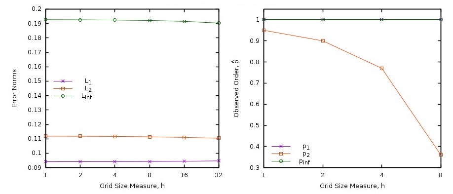
Fig. 2.4 Observed Temporal Order of Accuracy, MMS Solution to 1-D transient heat equation in MFIX¶

2.4.4.2. Spatial order of accuracy¶

Likewise, spatial order of accuracy is estimated by maintaining a constant time step, 0.005s in this case. On a spatial domain of \(\text{xϵ}\left\lbrack 0,1 \right\rbrack\), grid sizes were 3.12E-2m, 1.56E-2m, 7.81E-3m, 3.91E-3m and 1.95E-3m, resulting in a refinement factor, r, equal to 2. The observed order of accuracy, \(\widehat{p}\), converges to 2 which is equal to the formal order of the centered differencing scheme (diffusion term).

Table 2.10 L norms and the observed order for the unsteady heat equation – spatial order of accuracy 5¶
h	L ₁-norm	L ₂-norm	L _∞-norm	p (L ₁)	p (L ₂)	p (L _∞)
1	5.7762E-01	6.2875E-01	8.4644E-01	2.00	2.01	1.99
2	5.7783E-01	6.2884E-01	8.4627E-01	2.00	2.03	2.01
4	5.7867E-01	6.2920E-01	8.4559E-01	2.00	2.11	2.04
8	5.8204E-01	6.3068E-01	8.4285E-01	N/A	N/A	N/A
16	5.9554E-01	6.3708E-01	8.3158E-01	N/A	N/A	N/A

An example calculation, using h = 1, 2, 4 and \(L_{1}\)-norm is given:

\(\widehat{p} = \frac{\ln\left( \frac{\left\| \text{DE}_{\mathcal{l +}2} \right\| - \left\| \text{DE}_{\mathcal{l +}1} \right\|}{\left\| \text{DE}_{\mathcal{l +}1} \right\| - \left\| \text{DE}_{\mathcal{l}} \right\|} \right)}{\ln\left( r \right)} = \frac{\ln\left( \frac{\mathrm{5.7867E - 01} - \mathrm{5.7783E - 01}}{\mathrm{5.7783E - 01} - \mathrm{5.7762E - 01}} \right)}{\ln\left( \frac{\mathrm{3.12e - 2}}{\mathrm{1.56e - 2}} \right)} = 2.00\)

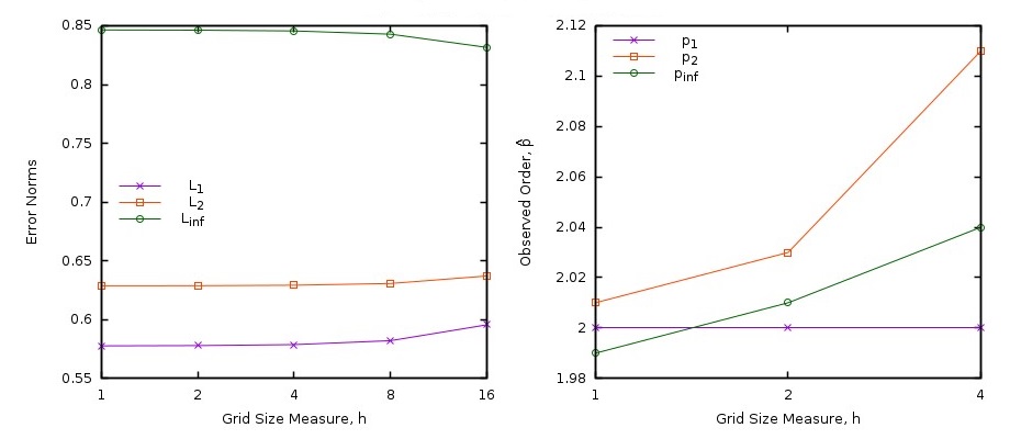
Fig. 2.5 Observed Spatial Order of Accuracy, MMS Solution to 1-D transient heat equation in MFIX¶

2.4.4.3. Combined order analysis¶

Having tested temporal and spatial discretization independently, a combined order analysis is performed by choosing grid size,\(\ \mathrm{\Delta}x\), and time step size, \(\mathrm{\Delta}t\), according to the descriptions in section 2.4.3. Based on the observed order of accuracies, it can be concluded that the energy equation in MFiX is reduced to a Forward Time Centered Space numerical scheme. In such a case, the pertinent non-dimensional number is the Fourier number given by,

(2.43)¶\[Fo = \ \alpha\frac{\mathrm{\Delta}t}{{\mathrm{\Delta}x}^{2}}\]

where \(\alpha\) represents a diffusivity constant.

The stability criterion for a Forward Time Centered Space scheme is \(Fo < \frac{1}{2}\). \(\text{Fo} = 0.32\) was chosen in this study, while \(\alpha\) is set to 1. The grid sizes used were 1.25E-1m, 6.25E-2m, 3.13E-2m, 1.56E-2m and 7.81E-3m. The corresponding time-step sizes are obtained as,

(2.44)¶\[\mathrm{\Delta}t = Fo\frac{{\mathrm{\Delta}x}^{2}}{\alpha}\]

Note that this observation is in complete agreement with the table presented in section 2.4.3 where the analysis expectation is a problem with spatial order equal 2, and temporal order equal 1, thereby producing \(r_{t} = \left( r_{x} \right)^{\frac{p}{q}} \rightarrow \mathrm{\Delta}t = Fo\left( \mathrm{\Delta}x \right)^{\frac{2}{1}}\) .

The orders of accuracy were calculated using Equations (2-42). The tables below show that the results from combined order analysis are consistent with the individual verification tests, giving a calculated observed temporal order, \(\widehat{q} = 1\) and a calculated observed spatial order, \(\widehat{p} = 2\).

Regardless of temporal or spatial analysis, the calculated norms used in combined order analysis are identical. This idea is illustrated in the following figure and tables.

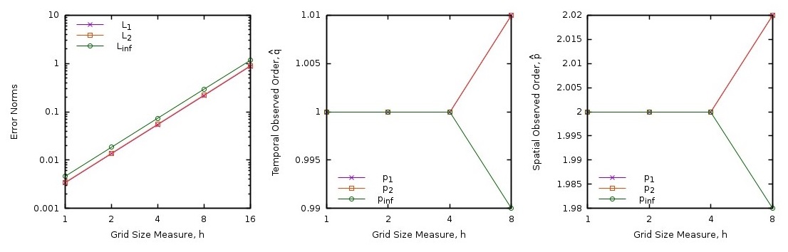
Fig. 2.6 Observed Temporal and Spatial Orders of Accuracy using Combined order analysis, MMS Solution to 1-D transient heat equation in MFIX¶

The key difference in calculation is the management of the denominator (related to refinement factor) for \(\widehat{q}\) and \(\widehat{p}\). As explained previously, in this case, the refinement factor for time is \(r_{t} = 4\), and the refinement factor for space is \(r_{x} = 2\).

Table 2.11 L norms and the observed order in combined order analysis for the unsteady heat equation – temporal order of accuracy¶
h	L ₁-norm	L ₂-norm	L _∞-norm	q (L ₁)	q (L ₂)	q (L _∞)
1	3.3848E-03	3.4552E-03	4.6133E-03	1.00	1.00	1.00
2	1.3542E-02	1.3823E-02	1.8453E-02	1.00	1.00	1.00
4	5.4204E-02	5.5336E-02	7.3780E-02	1.00	1.00	1.00
8	2.1741E-01	2.2202E-01	2.9422E-01	1.01	1.01	0.99
16	8.7873E-01	8.9901E-01	1.1638E+00	N/A	N/A	N/A

Table 2.12 L norms and the observed order in combined order analysis for the unsteady heat equation – spatial order of accuracy¶
h	L ₁-norm	L ₂-norm	L _∞-norm	p (L ₁)	p (L ₂)	p (L _∞)
1	3.3848E-03	3.4552E-03	4.6133E-03	2.00	2.00	2.00
2	1.3542E-02	1.3823E-02	1.8453E-02	2.00	2.00	2.00
4	5.4204E-02	5.5336E-02	7.3780E-02	2.00	2.00	2.00
8	2.1741E-01	2.2202E-01	2.9422E-01	2.02	2.02	1.98
16	8.7873E-01	8.9901E-01	1.1638E+00	N/A	N/A	N/A

An example calculation, using h = 2 and 4, with \(L_{1}\)-norm is given:

\[\widehat{q} = \frac{\ln\left( \frac{\mathrm{5.4204E - 02}}{\mathrm{1.3542E - 02}} \right)}{\ln\left( 4 \right)} = 1.00, \widehat{p} = \frac{\ln\left( \frac{\mathrm{5.4204E - 02}}{\mathrm{1.3542E - 02}} \right)}{\ln\left( 2 \right)} = 2.00\]

4: Significant digits shown in table may not result in shown values of \(\widehat{p}\) because of round-off error. If the reader runs these simulations and holds all significant digits for calculation, \(\widehat{p}\) values will match those shown.
5: Significant digits shown in table may not result in shown values of \(\widehat{p}\) because of round-off error. If the reader runs these simulations and holds all significant digits for calculation, \(\widehat{p}\) values will match those shown.