Steady Flow Around a Cylinder

This tutorial sets up fluid flow around a fixed circular cylinder based on the work of Schäfer et al. (1996). This is a steady, low-Reynolds-number cylinder-flow example that uses MFIX-Exa’s embedded-boundary geometry.

Features

• Incompressible fluid with no particles.

• Steady-state advance

• Quasi-2D domain using a thin, periodic spanwise direction.

• Cylinder represented by a predefined embedded boundary.

• Velocity inlet, pressure outlet, no-slip walls, and a periodic spanwise direction.

• Plotfile output for velocity, pressure, and EB volume fraction.

• Report output for the EB drag force.

Case description

The flow enters from the low-\(x=0.\) boundary and exits at the high-\(x=2.46\) boundary. The low-\(y=-0.20\) and high-\(y=0.21\) boundaries are no-slip walls. The cylinder has a radius of \(0.05\) m and is located at \(x=0.2\), \(y=0.\) so that it is slightly off-centered with respect to channel height. To mimic the original setup, the channel is thin and periodic in \(z\).

The tutorial uses

\[\rho = 1,\qquad \mu = 0.001,\qquad D = 0.1,\]

with the inlet velocity defined by

\[u(x=0,y) = \frac{1.2(y+0.2)(0.21-y)}{0.41^2} .\]

Defining the mean velocity as \(\overline{u} = 2u(x=0,y=0.41/2-0.2)/3 = 0.2\),

\[Re = \frac{\rho \overline{u} D}{\mu} = 20.\]

At this Reynolds number the wake should approach a steady, slightly-asymmetric state.

Important input sections

The mesh is a long box with a periodic \(z\) direction:

geometry.is_periodic =  0      0      1
geometry.prob_lo     =  0.00  -0.20  -0.205
geometry.prob_hi     =  2.46   0.21   0.205

amr.n_cell = 192  32  32

The cylinder is a predefined embedded boundary. The cylinder.internal_flow = false setting means the flow is outside the cylinder, not inside a pipe and the cylinder.height = -1.0 means that the cylinder is infinitely long:

mfix.geometry = "cylinder"

cylinder.internal_flow = false
cylinder.radius = 0.05
cylinder.height = -1.0
cylinder.direction = 2
cylinder.center = 0.2  0.0  0.0

The low- and high-\(y\) faces are no-slip walls. The low-\(x\) face is a mass inflow and the high-\(x\) face is a pressure outlet:

bc.regions =  bottom_wall  top_wall  inflow  outflow

bc.bottom_wall = no-slip
bc.top_wall = no-slip

bc.inflow = mi
bc.inflow.fluid.density = 1.0
bc.inflow.fluid.inflow_type = velocity
bc.inflow.fluid.velocity = "1.2*(y+0.2)*(0.21-y)/0.1681"

bc.outflow = po
bc.outflow.pressure = 101325.0

The case is run with the pseudo steady-state time advance with a tolerance of \(1.0e-6\) and 50,000 maximum iterations. The maximum time step size is set to ensure \(\Delta t \sim (\Delta x)^2\).

mfix.steady_state = 1

mfix.steady_state_tol = 1.0e-6
mfix.steady_state_maxiter = 50000

mfix.dt_max = 1.64e-4

Note

The complete input file is located in the MFIX-Exa source directory as tutorials/incompressible-fluid/inputs.steady-around-cylinder

Post-Processing

The run writes an AMReX plotfile named plt* every 5000 iterations into a directory, io, in the run directory. Each plot file saves the fluid:

• velocity field, vel_g,

• pressure, p_g, and

• embedded-boundary volume fraction, volfrac.

The plotfile data can be viewed in ParaView, VisIt, or any other AMReX-compatible post-processing tool. For visualization, load the final plt* directory and display the velocity magnitude on a slice normal to the spanwise direction. Overlaying velocity vectors helps show the acceleration around the cylinder and the steady wake behind it.

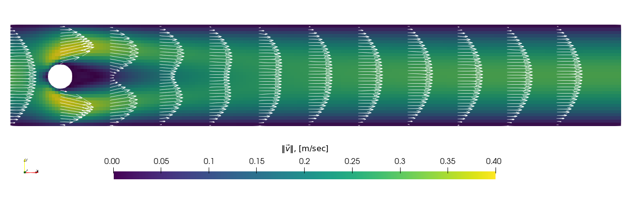
Fig. 11 Velocity magnitude and selected vector field at steady state.

The setup also enables the Embedded Boundary (EB) drag report for the EB surface captured by the eb_cyl region. This report region encloses the physical cylinder so that the EB surface is included in the integration; it does not redefine the cylinder geometry used by the flow solver.

regions = ... eb_cyl

regions.eb_cyl.shape = cylinder
regions.eb_cyl.cylinder.radius = 0.075
regions.eb_cyl.cylinder.start = 0.2  0.0  -0.205
regions.eb_cyl.cylinder.end   = 0.2  0.0   0.205

mfix.reports.eb_drag.regions = eb_cyl

mfix.reports.eb_drag.eb_cyl.int = 500

This report calculates the total aerodynamic force by integrating the fluid’s pressure and shear stress over the captured surface:

\[\vec{F} = \oint \left[-p\vec{n} + \vec{\tau} \cdot \vec{n} \right] dA\]

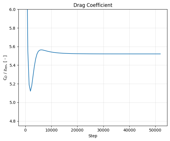
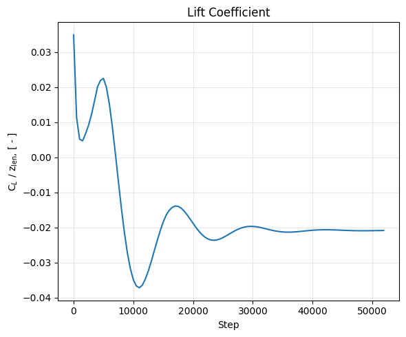
The report output is written every 500 iterations and contains the force components on the embedded boundary. For this two-dimensional benchmark, the streamwise force \(F_x\) is used to compute the drag coefficient and the cross-stream force \(F_y\) is used to compute the lift coefficient:

\[C_D = \frac{2 F_x}{\rho \overline{u}^2 D}, \qquad C_L = \frac{2 F_y}{\rho \overline{u}^2 D}.\]

Here \(D=0.1\) is the cylinder diameter and \(\overline{u}=0.2\) is the mean inlet velocity. At convergence, the coefficients should level off to nearly constant values, indicating that the steady-state solve has reached the expected asymmetric wake.

Fig. 12 Drag coefficient vs iteration

Fig. 13 Lift coefficient vs iteration

Extensions

• Refine amr.n_cell to run a uniformly finer mesh.

• Enable mesh refinement by increasing amr.max_level to refine the mesh near the embedded boundary

• Run at higher Reynolds number for longer times to observe unsteady vortex shedding.